2D points 3D Objects 3D Points Boundary Cursor position Data for selected object Domain Expansion Field Field components Field formula Field tubes Function Generate expansions along 2D boundary Generate expansions for 3D objects Grid formula Grid transformation Info and movie directives Insert Integral Modify 2D expansions MMP Movie Open GL window PET basis PFD (predefined FD) Project Space, plane, arrow, or point Tools and draw Transformation data Window
Press the integral button
![]() or
select Integral... from the Tools menu to
open this dialog.
or
select Integral... from the Tools menu to
open this dialog.
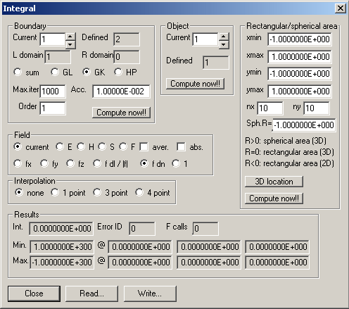
OpenMaXwell can evaluate integrals of the field either along a path in the xy plane, over a rectangular area in the xy plane, or over a 3D object. Boundaries are used as paths. I.e., boundaries play two different roles as 1) regular boundaries between two natural domains and 2) paths for computing integrals. These paths are ‘ineffective’ boundaries in most cases. They are usually within a single domain, i.e., the domain numbers to the left and right of the path are identical. Note that integrals are sometimes used in the MMP method for defining amplitudes. In this case, rough integral evaluations are sufficient in most cases.
Usually, OpenMaXwell integrates the current derived field (defined in the Field dialog). If you have not defined and computed the field to be integrated in the Field dialog, OpenMaXwell offers the chance to select one of the more frequently used fields, E, H, S, or F in the Field group. Moreover, you can decide whether you want to integrate the average of the field or not and whether OpenMaXwell shall sum up the absolute values (check the abs. box). Note that OpenMaXwell can also compute and integrate optical forces, when you select the F box. This only makes sense when the integration area coincides with the surface of a particle. Currently, particle procedures are only available for circular (2D) and spherical (3D) particles.
OpenMaXwell can either integrate one of the Cartesian components fx, fy, fz of a vector field (Scalar fields are considered as vector fields with an x component only!), a projection of the vector field f on the tangential direction (f dl - for boundary integrals only), the absolute value |f| of the vector field (except for boundary integrals), a projection on the normal direction (f dn), or the constant 1 (allows you to obtain the size of the integration area). Select the type in the corresponding box.
When you want to compute the integral along a path, you first have to define an ‘ineffective’ boundary with the tools for defining boundaries. In the Current box of the Boundary group, select the corresponding boundary number. If the boundary number is 0, the integrals over all boundaries are summed up. OpenMaXwell displays the number of boundaries that have been Defined and the domains to the left and to the right of this boundary in the L domain and R domain boxes respectively. When the L domain and R domain values are identical, or when the field in one of the domains is zero (domain number 0), the field in the non-zero field domain along the boundary will be computed. Otherwise, the field in both domains will be computed and the average of both values will be used for computing the integral.
OpenMaXwell has four methods for computing integrals. 1) sum: Simple summation in Max.iter points that are uniformly distributed. 2) GL: Non-adaptive Gauss-Legendre integration of a given Order. 3) GK: Adaptive Gauss-Kronrod and 4) adaptive HP integration. For adaptive integration, you specify not only the maximum number of function calls in the Max.iter box and the Order in the corresponding box, but also the desired accuracy in the Acc. Box.
When you want to integrate over a 2D rectangular area in the xy plane, you can specify the locations of the borders of the rectangle in the xmin, xmax, ymin, ymax boxes. In the Sph. R box you must enter any negative value, for example, -1.
When you specify 0 in the Sph. R box, OpenMaXwell integrates over a rectangular area that must be no longer in the xy plane. You may specify the location and orientation of this area in 3D space by pressing the 3D location button button.
When you specify a positive value R in the Sph. R box, OpenMaXwell integrates over the surface of a sphere with radius R. You may specify the location of the sphere in 3D space by pressing the 3D location button button.
Only simple summations on regular grids have been implemented so far. Therefore, you only have to specify the number of grid lines in the x and y directions in the nx and ny boxes. Note that these integrations are usually not very accurate.
When you want to integrate over the surface of a 3D object that is defined in the 3D Objects dialog, you can specify object number in the Current box of the Object group and press the corresponding Compute now!! button.
The derived field is known on a grid. Since the integration requires the evaluation also away from grid points, OpenMaXwell uses three types of interpolations. 1) 1 point: use the value in the closest grid points. 2) 3 point: get the three grid points that are closest to the current point and use linear interpolation. 3) 4 point: get the four grid points that are closest to the current point and use a bilinear interpolation. When the field is defined either by an analytic formula or by an MMP expansion, OpenMaXwell can evaluate the field anywhere and no interpolation is required. Select none in the Interpolation group when this is the case.
Press the Compute now!! button in the Boundary group when you want to evaluate a boundary integral or press the Compute now!! button in the Rectangular area group when you want to evaluate an integral on a rectangular area or in the Object area group for the evaluation of integrals over the surface of a 3D object. Note that the exclamation marks on these buttons indicate that the dialog will close.
When you compute boundary integrals, you can save the values of the integrand during the numeric integration in a function file. OpenMaXwell will ask you as soon as you press the Compute now!! Button in the Boundary group. This allows you to observe the integration process. If you select a simple summation, you obtain the field distribution along the boundary.
OpenMaXwell displays the results of the integration in the Info and movie directives dialog and in the corresponding group of the Integral dialog. Note that you cannot immediately read the output in the Results group because the Integral dialog closes when the evaluation of the integral starts. You have to open this dialog again to read the value of the integral, the error ID, and the number of F calls, i.e., of evaluations of the field required to obtain the result. This allows you to inspect the results when the corresponding output in the Info and movie directives dialog has been overwritten by another process. Note that an error ID unequal to zero indicates that the result is incorrect or at least not guaranteed to be as accurate as desired. OpenMaXwell also outputs information on the maximum and minimum values encountered during the integration on to the corresponding locations in 3D space.
Press the Read… button to read Integral data from a file. A file name dialog will allow you to select a file name to read from.
Press the Write… button to write Integral data to a file. A file name dialog will allow you to select a file name to save to.
Press the Close button to close the dialog. Note that the dialog’s data becomes effective once the dialog is closed.
Responsible for this web page: Ch. Hafner, Computational Optics Group, IEF, ETH, 8092 Zurich, Switzerland
Last update
17.02.2014