Cardiac DTI with off-resonance using a contracting LV with stylized background#
Summary#
Imports#
[ ]:
!pip install cmrseq==0.22.dev21 --index-url https://gitlab.ethz.ch/api/v4/projects/30300/packages/pypi/simple
!pip install cdtipy==2.4dev15 --index-url https://gitlab.ethz.ch/api/v4/projects/23794/packages/pypi/simple
!pip install cmr-rnd-diffusion==1.6 --index-url https://gitlab.ethz.ch/api/v4/projects/29882/packages/pypi/simple -q
!pip install cmr-widgets==0.6dev4 --index-url https://@gitlab.ethz.ch/api/v4/projects/37982/packages/pypi/simple -q
!pip install cmr-interpolation==1.5 --index-url https://gitlab.ethz.ch/api/v4/projects/29880/packages/pypi/simple -q
[2]:
import os
os.environ["TF_CPP_MIN_LOG_LEVEL"] = "3"

import tensorflow as tf
gpus = tf.config.list_physical_devices("GPU")
print(gpus)
if gpus:
    gpu_index = 0
    tf.config.set_visible_devices(gpus[gpu_index], "GPU")
    tf.config.experimental.set_memory_growth(gpus[gpu_index], True)

import ipywidgets
from IPython.display import display, HTML, Image, clear_output
import base64

import pyvista
import numpy as np
from tqdm.notebook import tqdm
import matplotlib.pyplot as plt
from pint import Quantity
%matplotlib widget

import sys
sys.path.insert(0, "../../")
sys.path.append("../")
import cdtipy
import cmr_widgets
import cmrseq

import cmrsim
import local_functions
[PhysicalDevice(name='/physical_device:GPU:0', device_type='GPU'), PhysicalDevice(name='/physical_device:GPU:1', device_type='GPU'), PhysicalDevice(name='/physical_device:GPU:2', device_type='GPU'), PhysicalDevice(name='/physical_device:GPU:3', device_type='GPU')]
/scratch/jweine/cdtipy/cdtipy/reconstruction.py:12: UserWarning: No matlab installation found!
  warnings.warn("No matlab installation found!")
/scratch/jweine/cdtipy/cdtipy/registration.py:14: UserWarning: No matlab installation found!
  warnings.warn("No matlab installation found!")
Prepare Background mesh#
Load static background configuration#
The snap-shots of the background mesh are provided in 50 ms intervals, where the peak systole is approximately at 350 ms. The Fourier-encoding defined later on, will assume this configuration. The example resource is given as short-axis view slices, but to compute the off-resonance induced by susceptibility gradients, the digital phantom has to be transformed into the scanner coordinate system. A simple rule-based assignment of tissue-susceptibilities according to the XCAT tissue labels is
performed inside the function local_functions.map_susceptibility_to_xcat_phantom
[2]:
bg_mesh = pyvista.read("../example_resources/NOR/XCAT_warped_vti/Image_07.vti")

# Transformation matrix (manually constructed)
matrix = np.array([[ 0.92541658, -0.35067681, -0.14363124,  0.        ],
                   [ 0.16317591,  0.02666648,  0.98623654,  0.        ],
                   [-0.34202014, -0.93611681,  0.08189961,  0.        ],
                   [ 0.        ,  0.        ,  0.        ,  1.        ]])

bg_mesh = local_functions.map_susceptibility_to_xcat_phantom(bg_mesh)
[3]:
Compute off-resonance#
As the spatial transformation in this case should not interpolate the scalar fields of the mesh (as done in mesh.transform) the points of the mesh acted on directly.
[32]:
new_bgmesh = bg_mesh.copy().cast_to_structured_grid()
augmented_points = np.concatenate([new_bgmesh.points, np.ones_like(new_bgmesh.points[:, 0:1])], axis=1)
new_bgmesh.points = np.einsum("ij, nj-> ni", matrix, augmented_points)[:, :3]
Now, a cmrseq-RegularGridDataset is instantiated from the mesh to use its functionality of calculating the off-resonance from the susceptibilty distribution (the intermediate result is saved to checkpoint the pre-processing).
[ ]:
grid_dataset = cmrsim.datasets.RegularGridDataset.from_unstructured_grid(new_bgmesh, pixel_spacing=Quantity([1, 1, 1], "mm"), padding=Quantity([3, 3, 3], "cm"))
grid_dataset.mesh.save("temp.vtk")
[ ]:
grid_dataset = cmrsim.datasets.RegularGridDataset(pyvista.read("temp.vtk"))
grid_dataset.compute_offresonance(Quantity(1.5, "T"), susceptibility_key="susceptibility");
[ ]:
grid_dataset.mesh.save("temp.vtk")
By intantiating the RegularGridDataset, the spatial susceptibility distribution is projected onto 3D grid with given spacing to facilitate the computation of off-resonance values per grid-point. To obtain the value corresponding to the original, unstructured background mesh the probe method is used. Furthermore, to avoid overwriting the mesh fields, a cleaned uniform mesh is instantiated that only contains the off-resonance field in units of millitesla
[33]:
grid_dataset = cmrsim.datasets.RegularGridDataset(pyvista.read("temp.vtk"))
offres_mesh = pyvista.UniformGrid(dimensions=grid_dataset.mesh.dimensions, spacing=grid_dataset.mesh.spacing, origin=grid_dataset.mesh.origin)
offres_mesh["deltaB0"] = grid_dataset.mesh["offres"]

new_bgmesh = offres_mesh.probe(new_bgmesh)
Save background as npz#
The loaded mesh also contains a voxelized version of the LV mesh obtained from biophysical simulation, which needs to filtered out for later use. Furthermore, only a slab of the phantom is extracted as the subsequent MR-simulation with diffusion contrast assumes a comparably small FOV. To allow for some simple breathing motion the extracted slab is still larger than the resulting image field of view.
The coordinates used to extract this slab are the short-axis view slice coordinates, where the base of the LV is located at \(\vec{r}=(0, 0, 0)^T\). Also, only the necessary mesh-arrays are saved to the npz file.
[ ]:
points_to_keep = np.where(np.sum([np.around(new_bgmesh["labels"]) == i for i in (0, 1, 2, 3, 4, 5, 6, 7, 8)], axis=0) < 0.5,
                          np.ones_like(new_bgmesh["labels"]), np.zeros_like(new_bgmesh["labels"]))
slice_thickness = Quantity(6, "cm")
slice_position = Quantity([0, 0, -5], "cm")
slice_normal = np.array([0, 0, 1])
fov_box = (0.35, 0.35)

points_in_box = np.where(np.stack([np.abs(bg_mesh.points[:, 0] - slice_position.m_as("m")[0]) < fov_box[0]/2,
                                   np.abs(bg_mesh.points[:, 1] - slice_position.m_as("m")[1]) < fov_box[1]/2,
                                   np.abs(np.einsum("pi, i", bg_mesh.points - slice_position.m_as("m")[np.newaxis], slice_normal)) <= slice_thickness.m_as("m") / 2]).prod(axis=0))
tmp_select = np.where(points_to_keep[points_in_box])

slice_data = pyvista.PolyData(bg_mesh.points[points_in_box][tmp_select])
for key in ["labels", "deltaB0", "PD", "T1", "T2", "labels"]:
    slice_data[key] = new_bgmesh[key][points_in_box][tmp_select]
[ ]:
np.savez("phantom_slice.npz",
         r_vectors=np.array(slice_data.points, dtype=np.float32),
         T1=np.array(slice_data["T1"], dtype=np.float32),
         T2=np.array(slice_data["T2"], dtype=np.float32),
         M0=np.array(slice_data["PD"], dtype=np.complex64),
         deltaB0=np.array(slice_data["deltaB0"], dtype=np.float32),
         labels=np.array(slice_data["labels"], dtype=np.int32)
        )
Calculate off-resonance on LV mesh#
[51]:
all_files = [os.path.abspath(f"../example_resources/NOR/VTK4Phantom/Displ{i:03}.vtk") for i in range(1, 24)]

timings = Quantity(np.arange(0, 23, 1) * 50, "ms")
cardiac_dataset = cmrsim.datasets.CardiacMeshDataset.from_list_of_meshes(all_files, timings, (4, 40, 30), field_key="displacement",)

refined_ds = cardiac_dataset.refine(6, 3, 5)
temp_mesh = refined_ds.mesh.copy()
temp_mesh.points = refined_ds.get_trajectories(Quantity(310, "ms"), Quantity(360, "ms"))[1].m_as("m")[:, 0]
augmented_coords = np.concatenate([temp_mesh.points, np.ones_like(temp_mesh.points[:, 0:1])], axis=1)
temp_mesh.points = np.einsum("ij, nj -> ni", matrix, augmented_coords)[:, :3]
lvmesh = offres_mesh.probe(temp_mesh)

refined_ds.mesh["deltB0_350.0ms"] = lvmesh["deltaB0"]
refined_ds.mesh.save("refined_lv.vtk")
Loading Files... : 100%|████████████████████████████████████████████████████████| 22/22 [00:00<00:00, 22.24it/s]
Refining mesh by factors: l=6, c=3, r=5: 100%|██████████████████████████████████| 23/23 [00:50<00:00,  2.21s/it]
Add diffusion tensors to LV#
This requires the installation of the custorm IBT-CMR python packages cmr-interpolation, cdtipy, cmr-widgets and cmr_rnd_diffusion.
More explanation on algorithm and implementation of sampling a random diffusion tensor distrubtion on 3D LV-meshes can be found on the cmr-random-diffmaps repository in the IBT-CMR Gitlab.
After executing this cell, the result can be rendered using this cell.
[36]:
sys.path.append("/scratch/jweine/cmr-random-diffmaps/")
import cmr_rnd_diffusion

cardiac_dataset = cmrsim.datasets.CardiacMeshDataset.from_single_vtk("refined_lv.vtk", mesh_numbers=((5-1)*4, 3*40+1, 6*30), time_precision_ms=1)
[cardiac_dataset.mesh.rename_array(f"displacements_{int(t)}ms", f"displacements_{t:1.1f}ms") for t in cardiac_dataset.timing];

points_at_350 = cardiac_dataset.get_positions_at_time(Quantity(350, "ms"))

cyl_coords = cmr_rnd_diffusion.mesh_utils.evaluate_cylinder_coordinates(cardiac_dataset.mesh.points.reshape(-1, 3), 16, 1+121*180)
local_basis = cmr_rnd_diffusion.diff3d.compute_local_basis(cardiac_dataset.mesh.points.reshape(-1, 3), mesh_numbers=(16, 180, 121))
ha = cmr_rnd_diffusion.diff3d.generate_ha(cyl_coords[..., 0], angle_range=(65, -65))
e2a = cmr_rnd_diffusion.diff3d.generate_e2a(cyl_coords, down_sampling_factor=50., seed_fraction=0.3, prob_high=0.4,
                                            high_angle_value=90., low_angle_value=1., kernel_width=0.25, distance_weights=(1., 1.5, 15.),
                                            verbose=True)
flat_eigenbasis = cmr_rnd_diffusion.diff3d.create_eigenbasis(np.stack([local_basis[k] for k in ["e_r", "e_c", "e_l"]], axis=-1).astype(np.float32), ha, e2a)
if os.path.exists("../example_resources/eigenvalue_pool.npy"):
    eigen_value_pool = np.load("../example_resources/eigenvalue_pool.npy")
else:
    with tf.device("CPU"):
        sampler = cmr_rnd_diffusion.sampling.MCRejectionSampler.from_savepath(f"../example_resources/sampler_diffusion_healthy_exp.npz",
                                                                              sampling_method=cmr_rnd_diffusion.sampling.exponentially_sample_simplex)
        eigen_value_pool = sampler.get_samples(50000)
        np.save("../example_resources/eigenvalue_pool.npy")
tensors = cmr_rnd_diffusion.diff3d.generate_tensors(np.repeat(eigen_value_pool, 4, axis=0), flat_eigenbasis, cyl_coords, seed_fraction=0.05,  kernel_variance=0.15)
np.save("temp_tensors.npy", tensors * (np.ones([3, 3]) + np.eye(3, 3) * 0.2)[np.newaxis]); clear_output();
MR-Simulation#
### Sequence definition
The MR-sequence is defined using the cmrseq package. In this case, one sequence object per diffusion weighting is created and stored in a python-list.
The resulting plot is created in this cell
[7]:
echo_time = Quantity(93, "ms")
fov = Quantity([21, 11.5], "cm") #* 2.5
sampling_matrix = (np.array([91, 49])).astype(int) #* 2 + 1

b_vectors = Quantity(np.loadtxt("../example_resources/bvectors.txt"), "s**(1/2)/mm")

seq_list = cmrseq.contrib.cardiac_diffusion.se_m012_ssepi(field_of_view=fov,
                                                          matrix_size=sampling_matrix,
                                                          echo_time=echo_time,
                                                          slice_thickness=Quantity(10., "mm"),
                                                          slice_pos_offset=Quantity(0, "m"),
                                                          b_vectors=b_vectors,
                                                          water_fat_shift="minimum",
                                                          spoiler_duration=Quantity(1.5, "ms"))

# Create copies that only contain the diffusion gradients with flipped decoding part
# as the phase tracking does not simulate the RF-pulse
diff_seq_list = [seq.copy() for seq in seq_list]
diff_seq_list = [seq.partial_sequence(copy_blocks=True, partial_string_match="diffusion", snap_to_raster=True) for seq in diff_seq_list]
[seq.shift_in_time(-seq.start_time) for seq in diff_seq_list]
[[b.scale_gradients(-1.) for b in seq.get_block(partial_string_match="decode")] for seq in diff_seq_list];

for seq in seq_list:
    seq._system_specs.grad_raster_time = Quantity(1, "us")
system_specs = seq_list[0]._system_specs
print(f"Resolution : {fov.to('mm')/sampling_matrix}")
Extending Sequence: 100%|██████████| 3/3 [00:00<00:00, 537.57it/s]
Max EPI duration: 41.599999999999994 millisecond
Resolution : [2.3076923076923075 2.3469387755102042] millimeter
/scratch/jweine/cmrseq/cmrseq/core/bausteine/_gradients.py:205: UserWarning: When calling snap_to_raster the waveform points are simply rounded to their nearestneighbour if the difference is below the relative tolerance. Therefore this in not guaranteed to be precise anymore
  warn("When calling snap_to_raster the waveform points are simply rounded to their nearest"
<IPython.core.display.Image object>
Instantiate Signal-models#
As mentioned before, two separate signal models (CompositeSignalModel instances) are used for fore-/background to incorporate motion induced phase only in the LV. The encoding module as well as some contrast operators are the same for both signal models, so they can be reused.
As the simulation is run for a single image per defined trigger-delay, the repetition dimension is not expanded between contrast operators. As the \(T_2^{*}\) weighting and \(B_0\) off-resonance operators expand the k-space axis, they are placed at the last positions to avoid redundant computations.
[8]:
# Encoding from Sequence definition
encoding_mod = cmrsim.analytic.encoding.GenericEncoding("encoding", seq_list[0], absolute_noise_std=[0., 1.], k_space_segments=sampling_matrix[1], device="GPU:0")
sampling_times = encoding_mod.sampling_times.read_value() - np.median(encoding_mod.sampling_times.read_value())

# Contrast Modules to compose signal model
off_mod = cmrsim.analytic.contrast.OffResonanceProperty(sampling_times, system_specs.gamma.m_as("1/mT/ms") * np.pi * 2, expand_repetitions=False)
coil_mod = cmrsim.analytic.contrast.BirdcageCoilSensitivities(map_shape=[*sampling_matrix, 1, 4], map_dimensions=[(-i/2, i/2) for i in fov.m_as("m") * 1.1] + [(-0.005, 0.005)], device="GPU:0")
se_mod = cmrsim.analytic.contrast.SpinEcho(echo_time=np.array([echo_time.m_as("ms"), ]) / 2, repetition_time=np.array([4000., ]), expand_repetitions=False)
t2_star = cmrsim.analytic.contrast.StaticT2starDecay(sampling_times, expand_repetitions=False)
diffusion_mod = cmrsim.analytic.contrast.GaussianDiffusionTensor(b_vectors=np.zeros([1, 3], dtype=np.float32), expand_repetitions=False)

grad_time, grad_wf = diff_seq_list[1].gradients_to_grid()
phase_tracking_wf = np.concatenate([grad_time[np.newaxis], grad_wf]).T[np.newaxis]
motion_mod = cmrsim.analytic.contrast.PhaseTracking(expand_repetitions=False, wave_form=phase_tracking_wf, gamma=system_specs.gamma_rad.m_as("rad/mT/ms"))

# Compose signal models for back/fore-ground
signal_model_bg = cmrsim.analytic.CompositeSignalModel(se_mod, diffusion_mod, coil_mod, off_mod)
signal_model_fg = cmrsim.analytic.CompositeSignalModel(se_mod, diffusion_mod, coil_mod, motion_mod, off_mod)
signal_model_fg_nomo = cmrsim.analytic.CompositeSignalModel(se_mod, diffusion_mod, coil_mod, off_mod)

print(signal_model_bg, "\n", signal_model_fg)
CompositeSignalModel:
        <cmrsim.analytic.contrast.sequences.SpinEcho object at 0x7f3993c2cc50>: spin_echo
        <cmrsim.analytic.contrast.diffusion_weighting.GaussianDiffusionTensor object at 0x7f3990e21610>: dti_gauss
        <cmrsim.analytic.contrast.coil_sensitivities.BirdcageCoilSensitivities object at 0x7f3990cfad90>: coil_sensitivities
        <cmrsim.analytic.contrast.offresonance.OffResonanceProperty object at 0x7f399057c410>: offres
 CompositeSignalModel:
        <cmrsim.analytic.contrast.sequences.SpinEcho object at 0x7f3993c2cc50>: spin_echo
        <cmrsim.analytic.contrast.diffusion_weighting.GaussianDiffusionTensor object at 0x7f3990e21610>: dti_gauss
        <cmrsim.analytic.contrast.coil_sensitivities.BirdcageCoilSensitivities object at 0x7f3990cfad90>: coil_sensitivities
        <cmrsim.analytic.contrast.phase_tracking.PhaseTracking object at 0x7f399101e390>: phase_tracking
        <cmrsim.analytic.contrast.offresonance.OffResonanceProperty object at 0x7f399057c410>: offres
### Set up Trajectory modules
The fore- and background are simulated separately as the foreground/left ventricle includes a contractile motion induced phase. Both back- and foreground are wrapped by the same breathing motion trajectory, to simulate respiratory-related displacements between shots. For simplicity a sinosidal breathing curve is assumed with a periodicity greater than the contracile motion perodicity of :math:1s.
The contractile motion is caputured by an instance of the PODTrajectoryModule using the provided LV-model snapshots.
Furthermore, a function to pick a subslice of the larger moving slab (background phantom) and the LV is defined below. This mimics an ideal slice-selective excitation. While this can also be implemented as contrast module probably involving higher computational cost, at this point a simple position-based slice-selection is performed.
An illustration of the moving, slice-selected background in combination with the full LV mesh is given below. The rendering is performed in this cell.
[9]:
@tf.function
def cut_phantomtf(phantom: dict, box_dimensions: list[float], xyz_to_mps: tf.constant = tf.eye(4, 4)):
    augmented_coords = tf.concat([phantom["r_vectors"], tf.ones_like(phantom["r_vectors"][:, 0:1])], axis=1)
    augmented_coords = tf.einsum('ij, pj -> pi', xyz_to_mps, augmented_coords)
    coords = augmented_coords[..., :3]
    in_x = tf.cast(tf.abs(coords[:, 0]) < tf.cast(box_dimensions[0], tf.float32) / 2, tf.float32)
    in_y = tf.cast(tf.abs(coords[:, 1]) < tf.cast(box_dimensions[1], tf.float32) / 2, tf.float32)
    in_z = tf.cast(tf.abs(coords[:, 2]) < tf.cast(box_dimensions[2], tf.float32) / 2, tf.float32)
    indices = tf.where(tf.reduce_prod(tf.stack([in_x, in_y, in_z], axis=0), axis=0))
    return {k:tf.gather(v, indices)[:, 0] for k, v in phantom.items()}
[30]:
cardiac_dataset = cmrsim.datasets.CardiacMeshDataset.from_single_vtk("refined_lv.vtk", mesh_numbers=(5*4, 3*40+1, 6*30), time_precision_ms=1)
[cardiac_dataset.mesh.rename_array(f"displacements_{int(t)}ms", f"displacements_{t:1.1f}ms") for t in cardiac_dataset.timing];
t_lv, r_lv = cardiac_dataset.get_trajectories(start=Quantity(-10, 'ms'), end=Quantity(1.5, 's'), string_cast=float)

# Instantiate module
contraction_mod = cmrsim.trajectory.PODTrajectoryModule(t_lv.m_as("ms"), r_lv.m_as("m"), n_modes=5,
                                                        poly_order=10, is_periodic=True, batch_size=50000)


#Wrap both background and contraction with breathing motion
breathing_amp = Quantity(1., "cm")
breathing_period = Quantity(3.1, "s")
breathing_direction = np.array([1, 2, 2])

breathing_mod = cmrsim.trajectory.SimpleBreathingMotionModule.from_sinosoidal_motion(cmrsim.trajectory.StaticParticlesTrajectory(),
                                                                                     breathing_period=breathing_period,
                                                                                     breathing_direction=breathing_direction,
                                                                                     breathing_amplitude=breathing_amp)

lv_trajectory_mod = cmrsim.trajectory.SimpleBreathingMotionModule.from_sinosoidal_motion(contraction_mod,
                                                                                         breathing_period=breathing_period,
                                                                                         breathing_direction=breathing_direction,
                                                                                         breathing_amplitude=breathing_amp)
clear_output()
<IPython.core.display.Image object>
Run simulation#
Below the two method for running the simulation loop are defined. The trigger-delays include the RR-interval duration but assumes the cardiac cylce to be exactly the same duration.
[32]:
tf.config.run_functions_eagerly(False)

def run_background_simulation(trigger_delays: np.ndarray, phantom_orig: dict[str, np.ndarray],
                              trajectory_mod: cmrsim.trajectory.BaseTrajectoryModule,
                              signal_model: cmrsim.analytic.CompositeSignalModel,
                              encoding_module: cmrsim.analytic.encoding.BaseSampling,
                              b_vectors: Quantity):
    """Runs the backgrodun simulation by looping over the trigger delays, calling the trajectory
    module, slicing the resulting phantom and updating the contrast-operator parameters if necessary.

    The parameters `trigger_delays` and `b_vectors` should have the same length, as a new diffusion weighting
    is selected for each trigger-delay.

    :returns: np.ndarray containing the flattened, complex k-space information
                with shape (#triggers, #coil, #noise-instance, #samples)
    """

    # Instantiate simulator and array to save k-space signal
    simulator = cmrsim.analytic.AnalyticSimulation("back_ground", building_blocks=[signal_model, encoding_module, None])
    kspaces_bg = np.zeros([n_trigger_delays, *simulator.get_k_space_shape().numpy().tolist()], dtype=np.complex64)
    for idx, triggers in tqdm(enumerate(trigger_delays), total=len(trigger_delays)):

        # Set diffusion weighting
        simulator.forward_model.dti_gauss.b_vectors.assign(b_vectors[idx:idx+1])

        # Get positions at echo time
        r_background, _ = trajectory_mod(initial_positions=phantom_orig["r_vectors"], timing=triggers[np.newaxis])
        ph = phantom_orig.copy()
        ph["r_vectors"] = r_background[:, 0].numpy()
        ph = cut_phantomtf(ph, box_dimensions=[*fov.m_as("m"), 0.01], xyz_to_mps=tf.constant([[1, 0, 0, 0], [0, 1, 0, 0],
                                                                                              [0, 0, 1, 0.03], [0, 0, 0, 1]]))
        # Add spherical diffusion tensors to background for fun-zees
        ph["diffusion_tensor"] = np.tile((np.eye(3, 3) * Quantity(5e-4, "mm**2/s").m).reshape(1, 3, 3),
                                         [ph["T1"].shape[0], 1, 1]).astype(np.float32)

        # Execute simulation and store results
        ds = cmrsim.datasets.AnalyticDataset(ph, filter_inputs=False, expand_dimension=True)
        kspaces_bg[idx] = simulator(ds, voxel_batch_size=40000).numpy()[..., 0, :]
    return kspaces_bg

def run_foreground_simulation(trigger_delays: np.ndarray, phantom: dict[str, np.ndarray],
                              trajectory_mod: cmrsim.trajectory.BaseTrajectoryModule,
                              signal_model: cmrsim.analytic.CompositeSignalModel,
                              encoding_module: cmrsim.analytic.encoding.BaseSampling,
                              b_vectors: Quantity, diff_seq_list: list[cmrseq.Sequence]) -> np.ndarray:
    """Runs the foreground simulation by looping over the trigger delays, calling the trajectory
    module, slicing the resulting phantom and updating the contrast-operator parameters if necessary.

    The parameters `trigger_delays` and `b_vectors` should have the same length, as a new diffusion weighting
    is selected for each trigger-delay.

    :returns: np.ndarray containing the flattened, complex k-space information
                with shape (#triggers, #coil, #noise-instance, #samples)
    """

    # Instantiate simulator and array to save k-space signal
    simulator = cmrsim.analytic.AnalyticSimulation("fore_ground", building_blocks=[signal_model, encoding_module, None])
    kspaces_fg = np.zeros([len(trigger_delays), *simulator.get_k_space_shape().numpy().tolist()], dtype=np.complex64)
    for idx, trig, seq_def in tqdm(zip(range(len(trigger_delays)), trigger_delays, diff_seq_list),
                                   total=len(trigger_delays)):

        # Set diffusion weighting
        simulator.forward_model.dti_gauss.b_vectors.assign(b_vectors[idx:idx+1])

        # Update Waveform for motion induced phase
        grad_time, grad_wf = seq_def.gradients_to_grid()
        phase_tracking_wf = np.concatenate([grad_time[np.newaxis], grad_wf]).T[np.newaxis]
        simulator.forward_model.phase_tracking.wave_form.assign(phase_tracking_wf)

        # Get initial positions at echo time
        r_foreground= np.concatenate([trajectory_mod(None, timing=trig[np.newaxis], batch_index=i)[0] for i in range(35)])

        # Batch-wise trajectory creation for motion induced motion (due to memory limitations)
        # Make sure the gradient time is correctly embedded into the global timing.
        # batch_size = trajectory_mod.sub_trajectory.batch_size.read_value()
        batch_size = trajectory_mod.batch_size.read_value()
        trajectories = np.empty([r_lv.shape[0], grad_time.shape[0], 3], dtype=np.float32)
        global_grad_time = (grad_time + trig - 70.).astype(np.float32)
        for i in tqdm(range(np.ceil(trajectories.shape[0] / batch_size).astype(np.int32)), leave=False):
            tr, _ = trajectory_mod(None, global_grad_time, batch_index=i)
            trajectories[i * batch_size : (i+1) * batch_size] = tr

        # Copy phantom, update motion related fields and cut out imaging slice
        ph = phantom.copy()
        ph["r_vectors"] = r_foreground[:, 0]
        ph["trajectory"] = trajectories
        ph = cut_phantomtf(ph, box_dimensions=[*fov.m_as("m"), 0.01], xyz_to_mps=tf.constant([[0, 1, 0, 0], [1, 0, 0, 0],
                                                                                              [0, 0, 1, 0.03], [0, 0, 0, 1]]))
        ph["M0"] *= 40000 / ph["M0"].shape[0]

        # Execute simulation and store results
        ds = cmrsim.datasets.AnalyticDataset(ph, filter_inputs=False, expand_dimension=True)
        kspaces_fg[idx] = simulator(ds, voxel_batch_size=50000).numpy()[..., 0, :]
    return kspaces_fg
[37]:
n_trigger_delays = 13
trigger_delays_ms = (np.arange(0, n_trigger_delays) * 1100 + 280).astype(np.float32)

bg_phantom = {k:v for k, v in np.load("phantom_slice.npz").items()}
bg_phantom["r_vectors"] += np.random.normal(0, 0.0003, bg_phantom["r_vectors"].shape)
# bg_phantom["r_vectors"] = bg_phantom["r_vectors"][:, (1, 0, 2)]
lbls = bg_phantom.pop("labels")

lv_phantom = dict(deltaB0=cardiac_dataset.mesh["deltB0_350.0ms"],
                  T1=np.ones_like(cardiac_dataset.mesh["deltB0_350.0ms"]) * 1000,
                  T2=np.ones_like(cardiac_dataset.mesh["deltB0_350.0ms"]) * 200,
                  M0=10*np.ones_like(cardiac_dataset.mesh["deltB0_350.0ms"]).astype(np.complex64),
                  diffusion_tensor=np.load("temp_tensors.npy") * 1e-3)

kspace_bg = run_background_simulation(trigger_delays_ms, bg_phantom, breathing_mod, signal_model_bg, encoding_mod, b_vectors); clear_output()
kspace_fg = run_foreground_simulation(trigger_delays_ms, lv_phantom, lv_trajectory_mod, signal_model_fg, encoding_mod, b_vectors, diff_seq_list); clear_output()

# kspace_fg = run_foreground_simulation(trigger_delays_ms, lv_phantom, contraction_mod, signal_model_fg, encoding_mod, b_vectors, diff_seq_list); clear_output()
# kspace_fg = run_foreground_simulation(trigger_delays_ms, lv_phantom, contraction_mod, signal_model_fg_nomo, encoding_mod, b_vectors, diff_seq_list); clear_output()
Reconstruction#
Import BART#
[13]:
import os
os.environ['TOOLBOX_PATH'] = "/scratch/shared/bart-master/"
os.environ['PATH'] = os.environ['TOOLBOX_PATH'] + ":" + os.environ['PATH']
sys.path.append(os.environ['TOOLBOX_PATH'] + "/python/")
import cfl
Estimate Coil-sensitivities#
Reconstruct the (diffusion-)unweighted images, using a NUFFT in BART and subsequently use this as input to the ECALIB sensitivity estimation.
[ ]:
_, k_vecs, _  = seq_list[0].calculate_kspace()
k_vecs = k_vecs.reshape(3, *sampling_matrix[::-1])
cfl.writecfl('bart_cfl/kcoord', k_vecs[:, :, :] / 2.8)

coil_images = []
coil_ksps = []
for coil_idx in tqdm(range(4)):
    ksp = (kspace_bg[0, coil_idx] + kspace_fg[0, coil_idx])
    cfl.writecfl('bart_cfl/kspace', ksp.reshape(1, *sampling_matrix[::-1]))
    !bart nufft -i -g -t -l 0.01 bart_cfl/kcoord bart_cfl/kspace bart_cfl/coil_image
    im = cfl.readcfl('bart_cfl/coil_image')[40:116, 52:97, :1]
    cfl.writecfl('bart_cfl/im_crop', im)
    coil_images.append(im)
    !bart fft 3 bart_cfl/im_crop bart_cfl/ksp_crop
    coil_ksps.append(cfl.readcfl('bart_cfl/ksp_crop'))
coil_images = np.stack(coil_images, axis=3)
coil_ksps = np.stack(coil_ksps, axis=2)[:, :, np.newaxis]

cfl.writecfl('bart_cfl/ecalib_in', coil_ksps)
!bart ecalib -m 1 -c 0 bart_cfl/ecalib_in bart_cfl/ecalib_out
sensitivities = cfl.readcfl('bart_cfl/ecalib_out')
clear_output();

# Plot results
plt.ioff(); plt.close("all")
f, axes = plt.subplots(4, 1, figsize=(10, 6))
ctmp = np.concatenate(coil_images[:, :, 0].transpose(2, 0, 1), axis=0)
stmp = np.concatenate(sensitivities[:, :, 0].transpose(2, 0, 1), axis=0)
axes[0].imshow(np.abs(ctmp).T[::-1], cmap="gray")
axes[1].imshow(np.angle(ctmp).T[::-1], cmap="twilight")
axes[2].imshow(np.abs(stmp).T[::-1], cmap="gray")
axes[3].imshow(np.angle(stmp).T[::-1], cmap="twilight")
f.tight_layout(); [_.axis("off") for _ in axes.flatten()]; f.subplots_adjust(wspace=0, hspace=0)
f.savefig("coil_sensitivity_estimation.png")
display(Image("coil_sensitivity_estimation.png"))
NUFFT Reconstruction per image and coil#
[38]:
# Calculate k-space weights
_, k_vecs, _  = seq_list[0].calculate_kspace()
clear_output()
k_vecs = k_vecs.reshape(3, *sampling_matrix[::-1])

os.makedirs("bart_cfl/", exist_ok=True)
cfl.writecfl('bart_cfl/kcoord', k_vecs[:, :, :] / 2.8)

# Reconstruct only foreground to obtain a LV-mask
ksp = kspace_fg[0, 0]
cfl.writecfl('bart_cfl/kspace', ksp.reshape(1, *sampling_matrix[::-1]))
!bart nufft -i -g -t bart_cfl/kcoord bart_cfl/kspace bart_cfl/adjoint_nufft


# # Reconstruct Both
bart_images = []
for tidx in tqdm(range(n_trigger_delays)):
    for coil_idx in range(4):
        # ksp = (kspace_bg[tidx, coil_idx] + kspace_fg[tidx, coil_idx])
        ksp = kspace_fg[tidx, coil_idx]
        cfl.writecfl('bart_cfl/kspace', ksp.reshape(1, *sampling_matrix[::-1]))

        !bart nufft -i -g -t -l 0.01 bart_cfl/kcoord bart_cfl/kspace bart_cfl/adjoint_nufft
        bart_images.append(cfl.readcfl('bart_cfl/adjoint_nufft')[..., 0])
bart_images = np.stack(bart_images, axis=0)
bart_images = bart_images.reshape(n_trigger_delays, -1, *bart_images.shape[1:])[..., :, 40:116, 52:97]
clear_output()
# print(bart_images.shape, mask_image.shape)
# np.save("bart_images.npy", bart_images)
mask_image = np.abs(cfl.readcfl('bart_cfl/adjoint_nufft')[40:116, 52:97, 0]) >  5e9
# np.save("bart_masks.npy", np.array(mask_image))
[39]:
np.save("bart_images_nobreathing.npy", bart_images)
# np.save("bart_images_nomotion.npy", bart_images)
mask_image = np.abs(cfl.readcfl('bart_cfl/adjoint_nufft')[40:116, 52:97, 0]) >  1e4
np.save("bart_masks_nobreathing.npy", np.array(mask_image))
# np.save("bart_masks_nomotion.npy", np.array(mask_image))
[20]:
plt.rcParams["font.family"] = "serif"

bart_images = np.load("bart_images.npy")[(0, 5, 7, 11), 0:1]
mask_image = np.load("bart_masks.npy")

# bart_images = np.load("bart_images_nobreathing.npy")[(0, 5, 7, 11), 0:1]
# mask_image = np.load("bart_masks__nobreathing.npy")
print(bart_images.shape, mask_image.shape)

abs_im = np.concatenate([np.concatenate(im, axis=-1) for im in np.abs(bart_images)], axis=0)
phase_im = np.concatenate([np.concatenate(im, axis=-1) for im in np.angle(bart_images)], axis=0)
mask_im = np.ma.masked_less(np.concatenate([np.concatenate([np.abs(mask_image), ] * bart_images.shape[1], axis=-1), ] * bart_images.shape[0], axis=0), 0.5)
print(mask_im.shape, abs_im.shape, phase_im.shape)

# plt.ioff(), plt.close("all")
# abs_im = np.concatenate([np.concatenate(im, axis=-1) for im in np.abs(bart_images)], axis=0)
# phase_im = np.concatenate([np.concatenate(im, axis=-1) for im in np.angle(bart_images)], axis=0)
# mask_im = np.ma.masked_less(np.concatenate([np.concatenate([mask_image, ] * bart_images.shape[1], axis=-1), ] * bart_images.shape[0], axis=0), 0.5)
# clear_output();


# Plot results
fill_str = " " * 37
sl = cmr_widgets.SlideShow(np.stack([abs_im.T, phase_im.T], axis=2), image_axes=(0, 1), row_axis=2,
                           cmaps=np.array([["gray"], ["twilight"]]),
                           clims=np.array([[dict(vmin=0, vmax=None)], [dict(vmin=-np.pi, vmax=np.pi)]]),
                           figure_kwargs=dict(figsize=(8, 3), constrained_layout=True),
                           titles=(f"$b_0${fill_str}$b_5${fill_str}$b_7${fill_str}$b_{{11}}$", ),
                           ylabels=("Magnitude", "Phase")
                           )
sl.figure.colorbar(sl.artists[1, 0], location="bottom", orientation="horizontal", shrink=0.9, pad=0.04, fraction=0.9, aspect=100, label="rad")
for i in range(4):
    cdtipy.plotting.mask_contour_overlay(sl.axes[0:1, 0], np.concatenate([np.zeros_like(mask_image.T), ]* i + [mask_image.T], axis=1),
                                         contour_kwargs={'edgecolor': (1, 0, 0, 1), 'facecolor': (1, 1, 1, 0), "linestyle":"--"})


sl.figure.savefig("NUFFT_BART_Reconstruction.svg")
sl.figure.savefig("Figure8.tiff", dpi=750)
# display(Image("NUFFT_BART_Reconstruction.png"))
(4, 1, 76, 45) (76, 45)
(304, 45) (304, 45) (304, 45)
(1, 45, 76) (1,)
(1, 45, 152) (1,)
(1, 45, 228) (1,)
(1, 45, 304) (1,)
Infer diffusion metrics#
The input to the tensor inference is data without breathing data. This is easily achievable by setting the motion amplitude of the SimpleBreathingModule to \(0 cm\)
[10]:
plt.rcParams["font.family"] = "serif"

sys.path.insert(0, "/scratch/jweine/cdtipy/")
import cdtipy

images = np.load("bart_images_nobreathing.npy")
images_ref = np.load("bart_images_nomotion.npy")
mask_images = np.stack([np.abs(np.load("bart_masks_nobreathing.npy")), np.load("bart_masks_nomotion.npy")], axis=0)

print(images.shape, mask_images.shape)
b_vecs = Quantity(np.loadtxt("../example_resources/bvectors.txt"), "s**(1/2)/mm")[1:][:, (1, 0, 2)]
b_vecs[:, :2] *= -1

bg_data = []
metrics_per_slice = []
for img, msk in zip([images, images_ref], mask_images):
    diff_in = np.sum(np.abs(img).transpose(2, 3, 0, 1), axis=-1, keepdims=True)[:, :, 1:]
    bg_data.append(diff_in)
    regressor = cdtipy.fitting.MatrixInversion(diff_in, b_vecs.m_as("s^(1/2)/mm"), mask=msk)
    regressor.fit()
    _, fit_tensors = regressor.get_result(dimensions=2)
    tensor_metrics = cdtipy.tensor_metrics.metric_set(fit_tensors)
    tensor_angulation = cdtipy.angulation.angulation_set(eigen_vectors=tensor_metrics["evecs"],
                                                         mask=msk, field_of_view=np.array([1, 1]))
    tensor_metrics["MD"][np.where(msk < 1)] = np.nan
    tensor_metrics["FA"][np.where(msk < 1)] = np.nan
    result_dict = dict(**tensor_metrics, **tensor_angulation)
    metrics_per_slice.append(result_dict)
bg_data = np.stack(bg_data, axis=2)
print(bg_data.shape)


plt.close("all")
figure, axes = cdtipy.plotting.layouts.metric_summary(figsize=(12, 8.5))
xlims = ((1.60e-3, 1.8e-3), (0.2, 0.38), (-60, 60), (0, 90))
slice_labels = ("No Motion", "Motion")
axes[1, 0].set_ylim([0, 0.15])
cdtipy.plotting.scalars.metric_maps(metrics_per_slice, #background_data=np.zeros_like(mask_images.transpose(1, 2, 0)),
                                     crop_percent=(0.2, 0.8, 0., 1.), axes=axes[2, :],
                                     masks=mask_images.transpose(1, 2, 0), clims=xlims,
                                     ylabel_spacing=40, slice_labels=slice_labels)
cdtipy.plotting.scalars.metric_histograms(metrics_per_slice, masks=mask_images,
                                          axes=axes[:2, :],
                                          add_text=True, plot_mean_std=False, xlims=xlims, slice_labels=slice_labels,
                                          hist_kw=dict(kde=True, facecolor=(0, 0, 0, 0), edgecolor=(0, 0, 0, 0), stat="probability"),
                                          text_anchor=(0.05, 0.94)
                                         );
# figure.savefig("dti_result_summary.svg")
figure.savefig("Figure10.tiff", dpi=500)
# figure.canvas

# clear_output();
# display(Image("dti_result_summary.png"))
(13, 4, 76, 45) (2, 76, 45)
100%|██████████| 372/372 [00:00<00:00, 29201.25it/s]
100%|██████████| 380/380 [00:00<00:00, 37709.64it/s]
(76, 45, 2, 12, 1)
Appendix - Rendering#
This chapter contains the code to create the figures/illustrations shown in this notebook.
Background mesh thresholding#
Uses the background mesh, aligned with the xyz-coordinate system, to create a surface-like rendering by thresholding
[ ]:
threshold_mesh = bg_mesh.copy().cast_to_structured_grid()
augmented_coords = np.concatenate([threshold_mesh.points, np.ones_like(threshold_mesh.points[:, 0:1])], axis=1)
threshold_mesh.points = np.einsum("ij, nj-> ni", matrix, augmented_coords)[:, :3]

threshold_mesh["labels"] = np.around(threshold_mesh["labels"], decimals=0)
threshold_mesh["islung"] = np.where(np.logical_or(threshold_mesh["labels"] == 15, threshold_mesh["labels"] == 16), np.ones_like(threshold_mesh["labels"]), np.zeros_like(threshold_mesh["labels"]))
threshold_mesh["isliver"] = np.where(threshold_mesh["labels"] == 13, np.ones_like(threshold_mesh["labels"]), np.zeros_like(threshold_mesh["labels"]))
threshold_mesh["isrib"] = np.where(threshold_mesh["labels"] == 31, np.ones_like(threshold_mesh["labels"]), np.zeros_like(threshold_mesh["labels"]))
threshold_mesh["islv"] = np.where(threshold_mesh["labels"] == 1, np.ones_like(threshold_mesh["labels"]), np.zeros_like(threshold_mesh["labels"]))
threshold_mesh["isrv"] = np.where(threshold_mesh["labels"] == 2, np.ones_like(threshold_mesh["labels"]), np.zeros_like(threshold_mesh["labels"]))

lung_mesh, liver_mesh, rib_mesh, lv_mesh, rv_mesh = [threshold_mesh.threshold(value=0.5, scalars=key) for key in ["islung", "isliver", "isrib", "islv", "isrv"]]

pyvista.close_all()
pyvista.start_xvfb()
plotter = pyvista.Plotter(off_screen=True, window_size=(300, 300))
plotter.add_mesh(lung_mesh, color="green")
plotter.add_mesh(liver_mesh, color="blue")
plotter.add_mesh(rib_mesh, color="yellow")
plotter.add_mesh(lv_mesh, color="red")
local_functions.add_custom_axes(plotter, scale=0.5)
plotter.screenshot("transformed_threshold_mesh_1.png");

plotter = pyvista.Plotter(off_screen=True, window_size=(300, 300))
plotter.add_mesh(lung_mesh, color="green")
plotter.add_mesh(liver_mesh, color="blue")
plotter.add_mesh(rib_mesh, color="yellow")
plotter.add_mesh(lv_mesh, color="red")
local_functions.add_custom_axes(plotter, scale=0.5)
plotter.camera.position = (0.15, -1., 0.4)
plotter.camera.focal_point = (-0.15, 1., -0.1)
plotter.camera.zoom(0.6)
plotter.screenshot("transformed_threshold_mesh_2.png");
Sliced Background mesh#
[ ]:
import matplotlib.pyplot as plt
N=30
base_cmap = 'cubehelix'
base = plt.colormaps.get_cmap(base_cmap)
color_list = base(np.linspace(0, 1, N))
cmap_name = base.name + str(N)
cmap = base.from_list(cmap_name, color_list, N)

pyvista.close_all()
pyvista.start_xvfb()
plotter = pyvista.Plotter(off_screen=True, window_size=(600, 300))
plotter.add_mesh(bg_mesh.slice_orthogonal(), scalars="labels", clim=(0, N), cmap=cmap)
plotter.screenshot("background_mesh_0.png");
[ ]:
import imageio
im1 = imageio.v3.imread("transformed_threshold_mesh_1.png")
im2 = imageio.v3.imread("transformed_threshold_mesh_2.png")
im3 = imageio.v3.imread("background_mesh_0.png")
print(im1.shape, im2.shape, im3.shape)
imcomb = np.concatenate([np.concatenate([im1, im2], axis=1), im3], axis=0)
imageio.v3.imwrite("background_mesh.png", imcomb)
Contracting LV-mesh#
Renders animation of contracting LV-mesh
[69]:
all_files = [os.path.abspath(f"../example_resources/NOR/VTK4Phantom/Displ{i:03}.vtk") for i in range(23)]
timings = Quantity(np.arange(0, 24, 1) * 50, "ms")

cardiac_dataset = cmrsim.datasets.CardiacMeshDataset.from_single_vtk("refined_lv.vtk", mesh_numbers=(4*4, 3*40+1, 4*30), time_precision_ms=1)
[cardiac_dataset.mesh.rename_array(f"displacements_{int(t)}ms", f"displacements_{t:1.1f}ms") for t in cardiac_dataset.timing];

pyvista.close_all()
pyvista.start_xvfb()
plotter = pyvista.Plotter(off_screen=True, window_size=(600, 600))
cardiac_dataset.render_input_animation("mesh", plotter)
[ ]:
pyvista.close_all()
pyvista.start_xvfb()
plotter = pyvista.Plotter(off_screen=True, window_size=(600, 600))
tmp_mesh = cardiac_dataset.mesh.copy()
plotter.add_mesh(tmp_mesh, color="gray");
plotter.screenshot("static_lv.png");
To execute the rendering in the cell below the code in the corresponding cell must be executed beforehand.
[66]:
import cdtipy
cardiac_dataset = cmrsim.datasets.CardiacMeshDataset.from_single_vtk("refined_lv.vtk", mesh_numbers=(4*4, 3*40+1, 4*30), time_precision_ms=1)
[cardiac_dataset.mesh.rename_array(f"displacements_{int(t)}ms", f"displacements_{t:1.1f}ms") for t in cardiac_dataset.timing];
tensors = np.load("temp_tensors.npy")
metric_set = cdtipy.tensor_metrics.metric_set(tensors * 1e-3)
cardiac_dataset.mesh["MD"] = metric_set["MD"][0]
cardiac_dataset.mesh["FA"] = metric_set["FA"][0]
cardiac_dataset.mesh["HA"] = ha
cardiac_dataset.mesh["E2A"] = e2a
cardiac_dataset.mesh["diffusion_tensors"] = tensors * 1e-3
pyvista.close_all()
def _add_chart(key: str, pl: pyvista.Plotter):
plt.close("all")
f_inlet, axes = plt.subplots(1, 1, figsize=(3, 3))
sns.histplot(cardiac_dataset.mesh.ptc()[key], ax=axes, kde=True, stat='frequency')
axes.set_xlabel(key)
axes.set_ylabel("frequency")
axes.set_yticks([])
axes.ticklabel_format(axis="x", style="sci", scilimits=(-2, 2))
f_inlet.subplots_adjust(bottom=0.22, top=0.9, left=0.01, right=0.95)
chart = pyvista.ChartMPL(f_inlet, size=(0.65, 0.26), loc=(0.175, 0.715))
chart.border_color = (1, 1, 1, 0)
chart.background_color = (1, 1, 1, 0)
pl.add_chart(chart)
def _add_mesh(key: str, pl: pyvista.Plotter, opacity: float, clim: tuple[float, float], cmap: str):
pl.add_mesh(cardiac_dataset.mesh.ptc(), scalars=key, cmap=cmap, opacity=mesh_opacity, clim=clim)
pl.add_mesh(cardiac_dataset.mesh.slice_orthogonal(), scalars=key, cmap=cmap, clim=clim)
pl.camera.position = (*pl.camera.position[0:2], pl.camera.position[2] + 0.03)
pl.camera.focal_point = (*pl.camera.focal_point [0:2], pl.camera.focal_point [2] + 0.03)
pyvista.start_xvfb()
plotter = pyvista.Plotter(off_screen=True, shape=(1, 4), window_size=(1200, 400))
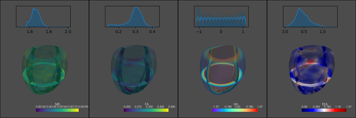
mesh_opacity = 0.25
plotter.subplot(0, 0)
_add_mesh("MD", plotter, mesh_opacity, clim=[1.3e-3, 1.9e-3], cmap="viridis")
_add_chart("MD", plotter)
plotter.subplot(0, 1)
_add_mesh("FA", plotter, mesh_opacity, clim=[0.2, 0.5], cmap="viridis")
_add_chart("FA", plotter)
plotter.subplot(0, 2)
_add_mesh("HA", plotter, mesh_opacity, clim=[-np.pi/2, np.pi/2], cmap="rainbow")
_add_chart("HA", plotter)
plotter.subplot(0, 3)
_add_mesh("E2A", plotter, mesh_opacity, clim=[0, np.pi/2], cmap="seismic")
_add_chart("E2A", plotter)
plotter.screenshot("tensor_example.png");
## Breathing motion & imaging slice
To execute the rendering in the cell below the code in the corresponding cell must be executed beforehand.
[92]:
fov = Quantity([21, 12], "cm") * 1.2

phantom_orig = {k:v for k, v in np.load("phantom_slice.npz").items()}
phantom_orig["r_vectors"] = phantom_orig["r_vectors"]#[:, (1, 0, 2)]

timing = np.linspace(0, 3600, 75).astype(np.float32)
trajectories = []
scalars = []
for t in tqdm(timing):
    r = breathing_mod(phantom_orig["r_vectors"], t[np.newaxis])[0]
    ph = phantom_orig.copy()
    ph["r_vectors"] = r[:, 0].numpy()
    ph = cut_phantomtf(ph, box_dimensions=[*fov.m_as("m"), 0.01], xyz_to_mps=tf.constant([[1, 0, 0, 0], [0, 1, 0, 0], [0, 0, 1, 0.03], [0, 0, 0, 1]]))
    r_lv_temp = lv_trajectory_mod(np.ones_like(r_lv[0].m.astype(np.float32)), t[np.newaxis])[0]
    trajectories.append(np.concatenate([ph["r_vectors"], r_lv_temp[:, 0]], axis=0))
    scalars.append(np.concatenate([ph["labels"], np.ones_like(r_lv_temp[:, 0, 0]) * 53], axis=0))

pyvista.start_xvfb()
plotter = pyvista.Plotter(off_screen=True, window_size=(600, 400))
local_functions.add_custom_axes(plotter, scale=0.1)
local_functions.animate_trajectories(plotter, trajectories, scalars=scalars, timing=timing,
                                     filename="combined_slice.gif", mesh_kwargs=dict(cmap="cubehelix"))
pyvista.close_all()
[92]:
True
[93]:
plt.close("all")
_t = np.linspace(0, 3200, 4000).astype(np.float32)
_triggers = (np.arange(0, 3) * 1100 + 350).astype(np.float32)

funci = contraction_mod._evaluate_trajectory(_t).numpy()
funci = np.stack([funci[i] for i in np.random.randint(10, 30000, size=10)])
print(funci.shape)
figure, axes = plt.subplots(2, 1, figsize=(6, 4))
axes[0].set_title("Contraction - random example trajectories")
axes[0].plot(_t, funci[..., 0].T)
axes[0].vlines(_triggers, *axes[0].get_ylim(), color="gray", alpha=0.5)

funci = breathing_mod(initial_positions=np.zeros([1, 3], dtype=np.float32), timing=_t)[0].numpy()
axes[1].set_title("Breathing trajectory")
axes[1].plot(_t, funci[..., 0].T)
axes[1].vlines(_triggers, *axes[1].get_ylim(), color="gray", alpha=0.5)
figure.tight_layout()
figure.savefig("trajectory_plots.png")
(10, 4000, 3)
[94]:
import imageio
_im1 = imageio.v3.imread("trajectory_plots.png")[np.newaxis, ..., :3]
_im2 = imageio.v3.imread("combined_slice.gif")
_imc = np.concatenate([_im2, np.tile(_im1, [_im2.shape[0], 1, 1, 1])], axis=2)
imageio.mimsave("combined_slice_and_plot.gif", _imc, duration=100, loop=0)
To execute the rendering in the cell below the code in the corresponding cell must be executed beforehand.
[6]:
import imageio
plt.ioff()

for idx, seq in tqdm(enumerate(seq_list), total=len(seq_list), leave=False):
    plt.close("all")
    figure = plt.figure(figsize=(12, 7))
    axes = figure.subplot_mosaic("AAABB;CCCBB")
    cmrseq.plotting.plot_sequence(seq_list[idx], axes=axes["A"], format_axes=True, add_legend=False);
    cmrseq.plotting.plot_block_names(seq_list[idx], axis=axes["C"]);
    cmrseq.plotting.plot_kspace_2d(seq_list[idx], ax=axes["B"], plot_raster_trajectory=False,
                                   map_sampling_times="relative", add_colorbar=True, colorbar_kwargs={"shrink":1., });
    figure.suptitle(f"Sequence #{idx}")
    figure.tight_layout()
    figure.savefig(f"seq_{idx:02}.png")

_mr_seq_def_pngs = [imageio.v3.imread(f"seq_{idx:02}.png") for idx in tqdm(range(len(seq_list)), leave=False)]
imageio.mimsave("mr_sequence_animation.gif", _mr_seq_def_pngs, duration=1000, loop=0)

for idx, _ in enumerate(seq_list):
    os.remove(f"seq_{idx:02}.png")
[72]:
plt.close("all")
figure, ax = plt.subplots(1, 1, figsize=(12, 6))
cmrseq.plotting.plot_sequence(seq_list[1], axes=ax, format_axes=True, add_legend=True)
figure.tight_layout()
# display(figure.canvas)
figure.savefig("sequence_def.png")
Backup#
[102]:
# print(kspaces_bg.shape, kspaces_fg.shape)
from skimage.morphology import closing, opening, dilation, erosion, disk

# recon_mod = cmrsim.reconstruction.Cartesian2D(sample_matrix_size=sampling_matrix[::-1], padding=((41, 41), (21, 21)))

# # Reconstruct only foreground to obtain a LV-mask
# ksp = kspace_fg[0, 0]
# kspace_corr = np.empty(sampling_matrix[::-1], np.complex64)
# kspace_flip_reverse = np.reshape(ksp, sampling_matrix[::-1])
# kspace_corr[::2] = kspace_flip_reverse[::2]
# kspace_corr[1::2] = kspace_flip_reverse[1::2, ::-1]
# mask_image = np.abs(recon_mod(kspace_corr.T.reshape(1, -1)).numpy()[0]) > 60
# mask_image = opening(mask_image)
# mask_image = np.ma.masked_less(mask_image, 0.5)


# images = []
# for idx in range(n_trigger_delays):
#     for coil_idx in range(4):
#         ksp = kspace_bg[idx, coil_idx] + kspace_fg[idx, coil_idx]
#         kspace_corr = np.empty(sampling_matrix[::-1], np.complex64)
#         kspace_flip_reverse = np.reshape(ksp, sampling_matrix[::-1])
#         kspace_corr[::2] = kspace_flip_reverse[::2]
#         kspace_corr[1::2] = kspace_flip_reverse[1::2, ::-1]
#         images.append(recon_mod(kspace_corr.T.reshape(1, -1)).numpy())
# images = np.concatenate(images, axis=0)
# images = images.reshape(n_trigger_delays, -1, *images.shape[1:])
# print(images.shape)
# np.save("images.npy", images)
# np.save("masks.npy", np.array(mask_image))

plt.ioff()
abs_im = np.concatenate([np.concatenate(im, axis=-1) for im in np.abs(images)], axis=0)
phase_im = np.concatenate([np.concatenate(im, axis=-1) for im in np.angle(images)], axis=0)
mask_im = np.ma.masked_less(np.concatenate([np.concatenate([mask_image, ] * images.shape[1], axis=-1), ] * images.shape[0], axis=0), 0.5)

f, axes = plt.subplots(2, 1, figsize=(17, 6))
axes[0].imshow(abs_im.T, cmap="gray")
axes[0].imshow(mask_im.T, cmap="jet", vmin=0, vmax=1, alpha=0.1)
axes[1].imshow(phase_im.T, cmap="twilight")
f.tight_layout()
f.savefig("stupid_reconstruction_images.png")
display(Image("stupid_reconstruction_images.png"))