Incorporating Motion in Analytic Simulations#
This notebooks demonstrates the mechanism by which motion is integrated into the simulation.
In the course of this demonstration the distinction between two types of motion is made: 1. Motion during the readout 2. Motion between the shots/repetitions
The reason for that is, that the way of passing motion information to the simulator differs for these to cases, while it can also be used jointly without any additional effort. Furthermore, the particle positions (isochromates that constitute the digitial phantom) can either be precomputed for all timings defined by the simualtion parameters, or being computed per batch. In both cases, the particle trajectories are captured by a cmrsim trajectory module.
The trajectories in this example are created by (in-plane) rotating and shifting a slice of a cylindrical phantom.
Content: 1. Imports 2. Define Simulator 3. Define static Phantom 3. Create Motion 4. Run Simulation 1. Motion between instananeous shots 2. Motion during readout
Imports#
[1]:
import sys
sys.path.insert(0, "../../")  # if cmrsim-repository was cloned -> import from there
sys.path.append("../")  # to import local_functions

import base64
from IPython.display import display, HTML, clear_output
from collections import OrderedDict
import math
from copy import deepcopy

import tensorflow as tf
tf.get_logger().setLevel('ERROR')
physical_devices = tf.config.list_physical_devices('GPU')
if physical_devices:
    print("Available GPUS: \n\t", "\n\t".join([str(_) for _ in physical_devices]))
    tf.config.experimental.set_visible_devices(physical_devices[0], 'GPU')
    tf.config.experimental.set_memory_growth(physical_devices[0], True)

from tqdm.notebook import tqdm
from pint import Quantity
import pyvista
import numpy as np
import imageio
import matplotlib.pyplot as plt
%matplotlib inline

import cmrsim
import local_functions
clear_output()
Define Simulator#
[2]:
from typing import Tuple

class ExampleSimulation(cmrsim.analytic.AnalyticSimulation):
    def build(self, matrix_size: Tuple[int, int] = (150, 150),
              field_of_view: Tuple[float, float] = (0.25, 0.3)):
        n_kx, n_ky = matrix_size

        # Encoding definition / To enable result comparisons, the noise is set to 0 here
        encoding_module = cmrsim.analytic.encoding.EPI(field_of_view=field_of_view, sampling_matrix_size=matrix_size,
                                                       read_out_duration=0.4, blip_duration=0.01, k_space_segments=n_ky,
                                                       absolute_noise_std=0.)
        # Signal module construction
        spinecho_module = cmrsim.analytic.contrast.SpinEcho(echo_time=tf.constant([50., 75, 100, 125]),
                                                            repetition_time=tf.constant([3000., 3000., 3000., 3000.]),
                                                            expand_repetitions=True)

        centered_times = tf.abs(encoding_module.sampling_times - tf.reduce_max(encoding_module.sampling_times) / 2)
        t2_star_module =  cmrsim.analytic.contrast.t2_star.StaticT2starDecay(centered_times, expand_repetitions=False)


        # Forward model composition
        forward_model = cmrsim.analytic.CompositeSignalModel(spinecho_module)

        # Reconstruction
        recon_module = cmrsim.reconstruction.Cartesian2D(sample_matrix_size=(n_kx, n_ky), padding=None)
        return forward_model, encoding_module, recon_module
[3]:
[0.002482269503546099 0.0024793388429752063] meter
/tmp/ipykernel_37066/3436044017.py:9: DeprecationWarning: Call to deprecated class EPI. (Consider using the cmrsim.analytic.encoding.GenericEncoding class incombination with a cmrseq.sequence definition)
  encoding_module = cmrsim.analytic.encoding.EPI(field_of_view=field_of_view, sampling_matrix_size=matrix_size,
Define static Phantom#
First the (sliced) cylindrical phantom is created by using a method from the local_function module. To illustrate the phantom, 3D renderings including the imaging slices are created and displayed below
[4]:
phantom_mesh = local_functions.create_cylinder_phantom(dimensions=(400, 400, 1), spacing=Quantity([0.5, 0.5, 10], "mm").m_as("m").tolist())
clear_output()
phantom_mesh
[4]:
| Header | Data Arrays | ||||||||||||||||||||||||||||||||||||||||||||||||||
|---|---|---|---|---|---|---|---|---|---|---|---|---|---|---|---|---|---|---|---|---|---|---|---|---|---|---|---|---|---|---|---|---|---|---|---|---|---|---|---|---|---|---|---|---|---|---|---|---|---|---|---|
|
|
[5]:
pyvista.close_all()
pyvista.start_xvfb()
plotter = pyvista.Plotter(window_size=(1500, 300), off_screen=True, shape=(1, 4))
for idx, sc in enumerate(["class", "M0", "T1", "T2"]):
    plotter.subplot(0, idx)
    plotter.add_mesh(phantom_mesh.copy(), scalars=sc)
    local_functions.add_custom_axes(plotter, scale=0.2)
    box = local_functions.transformed_box(reference_basis=np.eye(3, 3), slice_normal=np.array([0., 0., 1.]), readout_direction=np.array([1., 0., 0.]),
                                          slice_position=Quantity([0., 0., 0.], "m"), extend=Quantity([*field_of_view.m_as("m"), 0.01], "m"))
    plotter.add_mesh(box, color="white", opacity=0.2)
plotter.screenshot("phantom_example.png")
b64 = base64.b64encode(open("phantom_example.png",'rb').read()).decode('ascii')
display(HTML(f'<img src="data:image/gif;base64,{b64}" />'))
/scratch/jweine/cmrsim/notebooks/analytic_simulation/../local_functions.py:43: UserWarning: Optimal rotation is not uniquely or poorly defined for the given sets of vectors.
  rot, _ = Rotation.align_vectors(reference_basis, new_basis)

Create Motion#
Usually, cmrism assumes that a discretized trajectory is already available (e.g. obtained from displacement-fields at certain times). In this example a functional definition of the motion (rotation with constant velocity + periodic translation) is used to calculate such a discretized definition. To do so, the pyvista transform method for the phantom mesh is used.
[6]:
from scipy.spatial.transform import Rotation

time_grid = Quantity(np.arange(0, 501, 10), "ms")

# Define 24 full rotations about the phantom center over 6 seconds
rotation_angles = Quantity(2 * np.pi / time_grid[-1].m_as("ms") * time_grid.m_as("ms"), "rad")

# Define center-of-mass position doing one full oscilation in x-direction with amplitude 5cm in 6 seconds
com_xpos = np.sin(2 * np.pi / time_grid[-1].m_as("ms") * time_grid.m_as("ms")) * Quantity(5, "cm")

# Apply transformation matrix for each step and save positions
particle_trajectories = np.zeros([time_grid.shape[0], *phantom_mesh.points.shape])
for tidx, phi, x in tqdm(zip(range(time_grid.shape[0]), rotation_angles, com_xpos),
                         total=time_grid.shape[0], desc="Computing Tranformations..."):
    trafo_matrix = np.eye(4, 4)
    trafo_matrix[0:3, 0:3] = Rotation.from_rotvec(np.array([0., 0., 1]) * phi.m_as("rad")).as_matrix()
    trafo_matrix[0, 3] = x.m_as("m")
    m = phantom_mesh.transform(trafo_matrix, inplace=False)
    particle_trajectories[tidx] = m.points
    del m
Fit Trajectory module to capture motion at any given time
[7]:
trajectory_module = cmrsim.trajectory.TaylorTrajectoryN(time_grid=time_grid.m_as("ms"),
                                                        particle_trajectories=particle_trajectories.transpose([1, 0, 2]),
                                                        order=12)
fitted_trajectory, _ = trajectory_module(timing=time_grid.m_as("ms").astype(np.float32))
fitted_trajectory.shape
/scratch/jweine/conda/envs/tf29_pyvista/lib/python3.9/site-packages/numpy/polynomial/polyutils.py:656: RuntimeWarning: overflow encountered in square
  scl = np.sqrt(np.square(lhs).sum(1))
/scratch/jweine/conda/envs/tf29_pyvista/lib/python3.9/site-packages/numpy/polynomial/polynomial.py:1362: RankWarning: The fit may be poorly conditioned
  return pu._fit(polyvander, x, y, deg, rcond, full, w)
[7]:
TensorShape([129135, 51, 3])
Render animation of moving phantom#
[8]:
f, axes = plt.subplots(2, 1, sharex=True, figsize=(8, 5.6))
for i in range(0, 5):
    for j, a in enumerate(axes):
        if i==0:
            a.plot(time_grid.m, particle_trajectories[:, 1000 + i*10000, j], "x", color=f"C{i}", label="ref")
            a.plot(time_grid.m, fitted_trajectory[i*10000 + 1000, :, j], color=f"C{i}", linestyle="--", linewidth=1, label="fit")
        else:
            a.plot(time_grid.m, particle_trajectories[:, 1000 + i*10000, j], "x", color=f"C{i}")
            a.plot(time_grid.m, fitted_trajectory[i*10000 + 1000, :, j], color=f"C{i}", linestyle="--", linewidth=1)
axes[0].set_ylabel("x-coordinate")
axes[1].set_ylabel("y-coordinate")
axes[1].set_xlabel("Time [ms]")
f.suptitle("Example trajectories fo 5 points")
[a.legend() for a in axes]
f.savefig("coord_curves.png")
plt.close(f)

pyvista.start_xvfb()
box = local_functions.transformed_box(reference_basis=np.eye(3, 3), slice_normal=np.array([0., 0., 1.]), readout_direction=np.array([1., 0., 0.]),
                                      slice_position=Quantity([0., 0., 0.], "m"), extend=Quantity([*field_of_view.m_as("m"), 0.015], "m"))
plotter = pyvista.Plotter(off_screen=True, window_size=(400, 400))
local_functions.add_custom_axes(plotter, scale=0.2)
plotter.add_mesh(box, opacity=0.3)
plotter.add_title("Reference trajectories", font_size=6)
local_functions.animate_trajectories(plotter, trajectories=particle_trajectories,
                                     timing=time_grid.m_as("ms"),
                                     text_kwargs=dict(color="white", font_size=8),
                                     mesh_kwargs=dict(show_scalar_bar=False),
                                     filename="rotating_phantom.gif",
                                     scalars=[phantom_mesh["class"], ] * 51)
plotter = pyvista.Plotter(off_screen=True, window_size=(400, 400))
local_functions.add_custom_axes(plotter, scale=0.2)
plotter.add_mesh(box, opacity=0.3)
plotter.add_title("Fitted trajectories", font_size=6)
local_functions.animate_trajectories(plotter, trajectories=fitted_trajectory.numpy().transpose([1, 0, 2]),
                                     timing=time_grid.m_as("ms"),
                                     filename="rotating_phantom_fit.gif",
                                     text_kwargs=dict(color="white", font_size=8),
                                     mesh_kwargs=dict(show_scalar_bar=False),
                                     scalars=[phantom_mesh["class"], ] * 51)
clear_output()

refgif = imageio.v3.imread("rotating_phantom.gif")
fitgif = imageio.v3.imread("rotating_phantom_fit.gif")
img = imageio.v3.imread("coord_curves.png")
combined_gif = np.concatenate([refgif, fitgif, np.tile(img[np.newaxis, :400, :, :3], [len(fitgif), 1, 1, 1])], axis=2)
imageio.v3.imwrite("combined.gif", combined_gif, loop=100)
[9]:
b64 = base64.b64encode(open("combined.gif",'rb').read()).decode('ascii')
display(HTML(f'<img src="data:image/gif;base64,{b64}" />'))

Run Simulation#
For all motion cases below the mesh must be transformed into a dictionary of arrays of single precision. The required entry r_vectors is inserted, depending on the case
[10]:
flat_phantom = dict(M0=phantom_mesh["M0"].astype(np.complex64).reshape(-1, 1, 1),
                    T1=phantom_mesh["T1"].astype(np.float32).reshape(-1, 1, 1),
                    T2=phantom_mesh["T1"].astype(np.float32).reshape(-1, 1, 1),
                    T2star=phantom_mesh["T1"].astype(np.float32).reshape(-1, 1, 1))
Motion between shots#
(Results are shown jointly, after both simulations are run)
First, define the ‘trigger delay’ per shot in ms. The number of trigger-delays matches the number of TE/TR set inside the Simulator definition
[11]:
trigger_delays = Quantity([0, 50, 100, 150], "ms")
echo_times = simulator.forward_model.spin_echo.TE.read_value().numpy()
shot_timings = (trigger_delays.m_as("ms") + echo_times).astype(np.float32)
print("Times at Echo formation (relative to trajectory reference): ", shot_timings)
Times at Echo formation (relative to trajectory reference): [ 50. 125. 200. 275.]
Precomputed motion#
Call the trajectory module and reshape the results to match the defined input shape
[12]:
r_vectors_2shots = trajectory_module(shot_timings.astype(np.float32))[0].numpy()
r_vectors_2shots = r_vectors_2shots.reshape(-1, 4, 1, 3)
Copy the phantom-dictionary, insert the positions, create an AnalyticDataset instance and finally call the simulator
[13]:
ph_dict = deepcopy(flat_phantom)
ph_dict.update({"r_vectors": r_vectors_2shots})
print([f"{k}:{v.shape}" for k,v in ph_dict.items()])

dataset = cmrsim.datasets.AnalyticDataset(ph_dict, filter_inputs=True, expand_dimension=False)
%time simulated_images_1 = simulator(dataset, voxel_batch_size=20000)
['M0:(129135, 1, 1)', 'T1:(129135, 1, 1)', 'T2:(129135, 1, 1)', 'T2star:(129135, 1, 1)', 'r_vectors:(129135, 4, 1, 3)']
2022-12-22 09:34:03.882272: I tensorflow/core/grappler/optimizers/data/replicate_on_split.cc:32] Running replicate on split optimization
Run Simulation:         |XXXXXXXXXXXXXXX|127787/127787  |XXXXXXXXXXXXXXX|121/121 CPU times: user 11.6 s, sys: 2.43 s, total: 14 s
Wall time: 11.9 s
Using the trajectory Module#
[14]:
time_signatures = {"r_vectors": shot_timings.reshape(4, 1)}

non_trivial_indices = np.where(np.abs(phantom_mesh["M0"]) > 0)
tr_mod = cmrsim.trajectory.TaylorTrajectoryN(time_grid=time_grid.m_as("ms"),
                                             particle_trajectories=particle_trajectories.transpose(1, 0, 2)[non_trivial_indices].astype(np.float32),
                                             order=12, batch_size=20000)

ph_dict = deepcopy(flat_phantom)
ph_dict.update({"initial_positions": particle_trajectories[0].astype(np.float32)})

dataset = cmrsim.datasets.AnalyticDataset(ph_dict, filter_inputs=True, expand_dimension=False)

%time simulated_images_2 = simulator(dataset, voxel_batch_size=int(tr_mod.batch_size), trajectory_module=tr_mod, trajectory_signatures=time_signatures, additional_kwargs=dict())
/scratch/jweine/conda/envs/tf29_pyvista/lib/python3.9/site-packages/numpy/polynomial/polyutils.py:656: RuntimeWarning: overflow encountered in square
  scl = np.sqrt(np.square(lhs).sum(1))
/scratch/jweine/conda/envs/tf29_pyvista/lib/python3.9/site-packages/numpy/polynomial/polynomial.py:1362: RankWarning: The fit may be poorly conditioned
  return pu._fit(polyvander, x, y, deg, rcond, full, w)
2022-12-22 09:34:17.342045: I tensorflow/core/grappler/optimizers/data/replicate_on_split.cc:32] Running replicate on split optimization
Run Simulation:         |XXXXXXXXXXXXXXX|127787/127787  |XXXXXXXXXXXXXXX|121/121 CPU times: user 9.09 s, sys: 1.92 s, total: 11 s
Wall time: 9.49 s
Visualize simulation results side-by-side#
[15]:
for i, images in enumerate([np.squeeze(simulated_images_1), np.squeeze(simulated_images_2)]):
    magnitude, phase = np.abs(images), np.angle(images)
    fig, axes = plt.subplots(2, 4, figsize=(10, 5))
    axes[0, 0].set_ylabel("Magnitude")
    axes[0, 0].set_ylabel("Phase")

    for td, ax, im in zip(shot_timings, axes[0], magnitude):
        ax.imshow(im, cmap="gray", origin="lower")
        ax.axis("off")
        ax.set_title(f"Echo time: {td}")

    for ax, im in zip(axes[1], phase):
        ax.imshow(im, cmap="twilight", origin="lower")
        ax.axis("off")

    fig.suptitle(["Precomputed Motion", "Integrated Trajectory Module"][i], fontsize=15)
    fig.tight_layout()
    fig.savefig(f"temp{i}.png")
    plt.close(fig)
imageio.v3.imwrite("tempres.png", np.concatenate([imageio.v3.imread("temp0.png"), imageio.v3.imread("temp1.png")], axis=1))
b64 = base64.b64encode(open("tempres.png",'rb').read()).decode('ascii')
display(HTML(f'<img src="data:image/gif;base64,{b64}" />'))

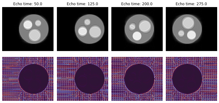
Motion during Readout#
Similar to the expansion of the r-vectors array in the previous section, motion in-between repetitions can be introduced by changing the #repetitions axis of the position vectors. Although for virtually any non-toy-example imaging matrix with e.g. (100, 100) = (10000) entries, precomputing the motion for ~1e5 particles becomes unpractical and the simulation time will be dominated by the IO limitations. Therefore, in this case we only use the batch-wise computation of positions that can also
use GPU.
Run#
[16]:
trigger_delays = Quantity([0, 50, 100, 150], "ms")
echo_times = simulator.forward_model.spin_echo.TE.read_value().numpy()
shot_timings = (trigger_delays.m_as("ms") + echo_times).astype(np.float32)
sampling_times = simulator.encoding_module.sampling_times.read_value().numpy().astype(np.float32)
time_signatures = {"r_vectors": sampling_times.reshape(1, -1) + shot_timings.reshape(4, 1)}
print(time_signatures["r_vectors"].shape)

non_trivial_indices = np.where(np.abs(phantom_mesh["M0"]) > 0)
tr_mod = cmrsim.trajectory.TaylorTrajectoryN(time_grid=time_grid.m_as("ms"),
                                             particle_trajectories=particle_trajectories.transpose(1, 0, 2)[non_trivial_indices].astype(np.float32),
                                             order=12, batch_size=2500)

ph_dict = deepcopy(flat_phantom)
ph_dict.update({"initial_positions": particle_trajectories[0].astype(np.float32)})

dataset = cmrsim.datasets.AnalyticDataset(ph_dict, filter_inputs=True, expand_dimension=False)

for i, b in dataset(batchsize=int(tr_mod.batch_size)).enumerate().take(1):
    b = simulator._map_trajectories(i, b, trajectory_module=tr_mod, trajectory_signatures=time_signatures, additional_kwargs=dict())
    print(i, [f"{k}: {v.shape}" for k, v in b.items()])

%time simulated_images_3 = simulator(dataset, voxel_batch_size=int(tr_mod.batch_size), trajectory_module=tr_mod, trajectory_signatures=time_signatures, additional_kwargs=dict())
(4, 17061)
2022-12-22 09:34:38.690233: I tensorflow/core/grappler/optimizers/data/replicate_on_split.cc:32] Running replicate on split optimization
tf.Tensor(0, shape=(), dtype=int64) ['M0: (2500, 1, 1)', 'T1: (2500, 1, 1)', 'T2: (2500, 1, 1)', 'T2star: (2500, 1, 1)', 'r_vectors: (2500, 4, 17061, 3)']
2022-12-22 09:34:39.149664: I tensorflow/core/grappler/optimizers/data/replicate_on_split.cc:32] Running replicate on split optimization
Run Simulation:         |XXXXXXXXXXXXXXX|127787/127787  |XXXXXXXXXXXXXXX|121/121 CPU times: user 49.2 s, sys: 9.83 s, total: 59 s
Wall time: 23 s
Display Results#
[17]:
simulated_images_3 = np.squeeze(simulated_images_3)
magnitude, phase = np.abs(simulated_images_3), np.angle(simulated_images_3)
fig, axes = plt.subplots(2, 4, figsize=(10, 5))
axes[0, 0].set_ylabel("Magnitude")
axes[0, 0].set_ylabel("Phase")

for td, ax, im in zip(shot_timings, axes[0], magnitude):
    ax.imshow(im, cmap="gray", origin="lower")
    ax.axis("off")
    ax.set_title(f"Echo time: {td}")

for ax, im in zip(axes[1], phase):
    ax.imshow(im, cmap="twilight", origin="lower")
    ax.axis("off")

fig.tight_layout()