Turbulent Flow Trajectories#
This notebook demonstrates the usage of the TurbulentTrajectory class to generate particle trajectorie within a flow field containing Reynolds-stress tensors. The positional updates are performed according to the Langevin equation.
Imports#
[ ]:
!pip install cmrseq --index-url https://gitlab.ethz.ch/api/v4/projects/30300/packages/pypi/simple
[1]:
# Load TF and check for GPUs
import os
os.environ['TF_CPP_MIN_LOG_LEVEL'] = '2'
import tensorflow as tf
gpus = tf.config.list_physical_devices('GPU')
for gpu in gpus:
    tf.config.experimental.set_memory_growth(gpu, True)
tf.config.set_visible_devices(gpus[1], "GPU")
logical_gpus = tf.config.list_logical_devices('GPU')
print(len(gpus), "Physical GPUs,", len(logical_gpus), "Logical GPUs")

# 3rd Party dependencies
from pint import Quantity
import pyvista
import numpy as np
import matplotlib.pyplot as plt
from matplotlib import cm
from copy import deepcopy
from tqdm.notebook import tqdm
from time import perf_counter

# Project library cmrsim
import sys
sys.path.insert(0, "../..")
import cmrsim
import cmrsim.utils.particle_properties as part_factory
4 Physical GPUs, 1 Logical GPUs
Define positions of slice and refilling volume#
[2]:
dt = Quantity(0.01,"ms")
TR = Quantity(5,"ms")
num_TR = 50

# Define Reseeding slice parameters
seeding_slice_position = Quantity([0, 0.048, -0.045], "m")
seeding_slice_normal = np.array([1., 0., 0.])
seeding_slice_thickness = Quantity(50, "mm")
seeding_pixel_spacing = np.array((0.25e-3, 0.25e-3, 0.25e-3)) # resolution of seeding mesh, mm
seeding_slice_bb = Quantity([5, 5.1, 2], "cm")
seeding_particle_density = 3 # per 1/mm*3

# Define initial filling
initial_fill_normal = np.array([1., 0., 0.])
initial_fill_position = Quantity([-0.0005, 0., 0.], "m")
initial_fill_thickness = Quantity(50, "mm")
initial_fill_bounding_box = Quantity([25, 25, 25], "cm")
lookup_mesh_spacing = np.array((0.5e-3, 0.5e-3, 0.5e-3)) # resolution of lookup mesh, mm


steps_per_TR = int(np.round(TR/dt).m_as("dimensionless"))
Load UBend mesh#
First load the mesh and aling along z#
[3]:
# Load UBend Example.
mesh = pyvista.read("../example_resources/sUbend_219_9.vtu")

# The velocity [m/s] is stored in the mesh as U1. In cmrsim all definitions are done in [ms] therefore
# We add the velocity field as scaled data to the mesh
mesh["velocity"] = Quantity(mesh["U"], "m/s").m_as("m/ms")
mesh.points = mesh.points[:,[2,1,0]]
mesh["velocity"] = mesh["velocity"][:,[2,1,0]]
mesh["RST"] = mesh["RST"][:,[5,4,2,3,1,0]]
mesh["Reflectionmap"] = mesh["U"][:,0]*0 + 1 # in ms
tfreq = np.sqrt(np.sum(mesh["RST"][:,[0,3,5]],1));
tfreq = tfreq / np.percentile(tfreq,90) * 1000
mesh["Frequency"] = tfreq # in Hz
Convert Reynolds stress tensor into cholesky decomposition#
[4]:
mesh["RST"] = mesh["RST"] # m^2/s^2
# RST form xx xy xz yy yz zz

a11=np.sqrt(np.clip(mesh["RST"][:,0],0,None) + np.min(np.abs(mesh["RST"][:,0])))
a21=mesh["RST"][:,1]/a11
a22=np.sqrt(np.clip(mesh["RST"][:,3]-a21**2,0,None) + np.min(np.abs(mesh["RST"][:,3]-a21**2)))
a31=mesh["RST"][:,2]/a11
a32=(mesh["RST"][:,4]-a21*a31)/a22
a33=np.sqrt(np.clip(mesh["RST"][:,5]-a31**2-a32**2,0,None))

# Chol form
mesh["chol"] = np.stack([a11,a21,a22,a31,a32,a33],axis=1)/1000 # m/ms

global_mesh_offset = [0, 0.04, -0.05]
mesh.translate(global_mesh_offset, inplace=True)
mesh = mesh.cell_data_to_point_data()
# clip to restricted length to reduce mesh-size
mesh.clip(normal='-z', origin=[0., 0., -0.1], inplace=True)
print(np.percentile(np.sqrt(np.sum(mesh["RST"][:,[0,3,5]],1)),90))
0.8562077098606697
Instantiate RefillingFlowDataset#
[5]:
# setup initial fill dict
initial_fill_dict = {'slice_normal':initial_fill_normal,
                     'slice_position':initial_fill_position.m_as('m'),
                     'slice_thickness':initial_fill_thickness.m_as('m'),
                     'slice_bounding_box':initial_fill_bounding_box.m_as('m')}

# Setup flow dataset with seeding mesh information
particle_creation_fncs = {}

dataset = cmrsim.datasets.RefillingFlowDataset(mesh,
                                               particle_creation_callables=particle_creation_fncs,
                                               slice_position=seeding_slice_position.m_as("m"),
                                               slice_normal=seeding_slice_normal,
                                               slice_thickness=seeding_slice_thickness.m_as("m"),
                                               slice_bounding_box=seeding_slice_bb.m_as("m"),
                                               lookup_map_spacing=lookup_mesh_spacing,
                                               seeding_vol_spacing=seeding_pixel_spacing,
                                               field_list=[("velocity", 3), ("chol",6),("Frequency",1),("Reflectionmap",1)])
mesh
/opt/conda/lib/python3.11/site-packages/pyvista/core/grid.py:873: PyVistaDeprecationWarning: `UniformGrid` is deprecated. Use `ImageData` instead.
  warnings.warn(
Updated Mesh
/opt/conda/lib/python3.11/site-packages/pyvista/core/grid.py:873: PyVistaDeprecationWarning: `UniformGrid` is deprecated. Use `ImageData` instead.
  warnings.warn(
Updated Slice Position
[5]:
| Header | Data Arrays | ||||||||||||||||||||||||||||||||||||||||||||||||||||||||||||||
|---|---|---|---|---|---|---|---|---|---|---|---|---|---|---|---|---|---|---|---|---|---|---|---|---|---|---|---|---|---|---|---|---|---|---|---|---|---|---|---|---|---|---|---|---|---|---|---|---|---|---|---|---|---|---|---|---|---|---|---|---|---|---|---|
|
|
Instantiate trajectory module#
[6]:
lookup_table_3d, map_dimensions = dataset.get_lookup_table()
trajectory_module = cmrsim.trajectory.TurbulentTrajectory(velocity_field=lookup_table_3d.astype(np.float32),
                                                          map_dimensions=map_dimensions.astype(np.float32),
                                                          additional_dimension_mapping=dataset.field_list[3:],
                                                          device="GPU:0")
Illustration 1 - Randomly seeded starts#
Run trajectory simulation#
[7]:
# Save subset of trajectories
traj = []

npart = 250
tracking_inds = (np.round(np.random.uniform(0,1,[npart,])*20000).astype(np.int32)).tolist()

traj = np.zeros([npart,steps_per_TR*num_TR+1,3])

# Initial fill

r, _ = dataset.initial_filling(particle_density=seeding_particle_density, slice_dictionary=initial_fill_dict)

save_inds = list(range(np.shape(tracking_inds)[0]))

trajectory_module.warmup_step(particle_positions=r)

traj[:,0,:] = r[tracking_inds,:]
cur_dt = 1

pbar = tqdm(range(num_TR), desc="Running Trajectory Sim", leave=True)
for tr in pbar:

    start = perf_counter()

    r_new = r
    pbar2 = tqdm(range(steps_per_TR), desc="Internal TR loop", leave=False)
    # Increment over TR
    for _ in pbar2:

        r_new, _ = trajectory_module.increment_particles(r_new, dt.m_as("ms"))
        traj[save_inds,cur_dt,:] = r_new.numpy()[tracking_inds,:]
        cur_dt = cur_dt+1

    displacements = np.linalg.norm(r - r_new, axis=-1) * 1000
    mid = perf_counter()

    # Reseed
    r, _, in_tol = dataset(particle_density=seeding_particle_density,
                           residual_particle_pos=r_new.numpy(),
                           distance_tolerance=0.2,
                           reseed_threshold=1)
    removed_idx = []
    for ind, idx in zip(tracking_inds,range(len(tracking_inds))):

        new_ind = np.argwhere(in_tol[0]==ind) # find its new index
        if new_ind.shape[0]==0: # check if particle is culled
            removed_idx.append(idx)
        else: # if not, update index
            tracking_inds[idx] = new_ind[0][0]

    for ele in sorted(removed_idx, reverse = True):
        del tracking_inds[ele]
        del save_inds[ele]


    n_new = dataset.n_new
    trajectory_module.turbulence_reseed_update(in_tol, new_particle_positions=r[-n_new:, :])

    end = perf_counter()
    n_reused_particles = in_tol[0].shape[0] if in_tol is not None else 0
    pbar.set_postfix_str(
        f"Particles Reused: {n_reused_particles}/{r.shape[0]}  // "
        f" New vs. Drop: {n_new}/{dataset.n_drop}  // "
        f" Density: {dataset.mean_density: 1.3f}/mm^3 // "
        f" Durations: {mid - start:1.3f} | {end - mid:1.3f} // "
        f" Displacements: {np.median(displacements):1.1f},({np.percentile(displacements,97):1.2f},{np.percentile(displacements,3):1.2f}) mm"
    )
[10]:
np.savez("illustration_1.npz", r_final=r, trajectory=traj)
Plot results#
[ ]:
%matplotlib inline
plt.close("all")
fig, axes = plt.subplots(1, 2, figsize=(18, 8))
A, xe, ye, _ = axes[0].hist2d(r[:,1],r[:,2], 600)
axes[0].clear()

for tr in range(traj.shape[0]):
    curtraj = traj[tr,:,:]
    trajlen = np.count_nonzero(np.sum(np.abs(curtraj),axis=1))
    axes[1].plot(np.trim_zeros(curtraj[:,2]), np.trim_zeros(curtraj[:,1]),
                 c=cm.hot(np.clip(trajlen/(steps_per_TR*num_TR),0,1)))

axes[0].imshow(A, vmax=5, extent=[ye.min(),ye.max(),xe.max(),xe.min()]);
axes[1].imshow(A, vmax=5, extent=[ye.min(),ye.max(),xe.max(),xe.min()]);
axes[0].set_title("Final particle density");
axes[1].set_title("Particle trajectories")
fig.tight_layout()
Plot 2D histogram#
[ ]:
fig, ax = plt.subplots(1, 1, figsize=(6, 6), constrained_layout=True)
A, xe, ye, _ = axes[0].hist2d(r[:,1],r[:,2], 600)
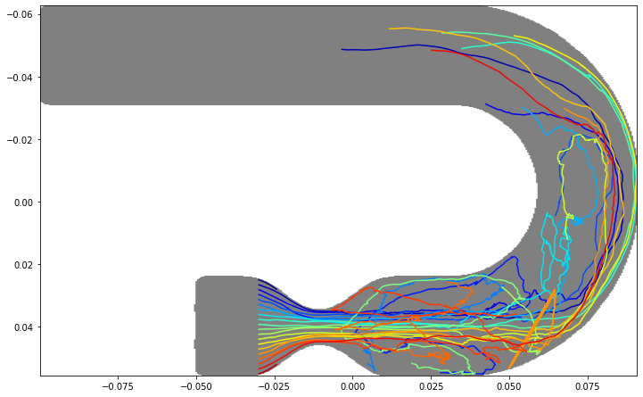
Illustration 2 - Starting positions in a line#
[173]:
# save initial fill for later only
r_initial, _ = dataset.initial_filling(particle_density=10, slice_dictionary=initial_fill_dict)
[174]:
lookup_table_3d, map_dimensions = dataset.get_lookup_table()
trajectory_module = cmrsim.trajectory.TurbulentTrajectory(velocity_field=lookup_table_3d.astype(np.float32),
                                                          map_dimensions=map_dimensions.astype(np.float32),
                                                          additional_dimension_mapping=dataset.field_list[3:],
                                                          device="GPU:0")
Simulate trajectories#
[175]:
steps = int(np.round(num_TR*TR/dt).m_as("dimensionless"))
r, properties, _ = dataset(seeding_particle_density)
npart = 20
r = np.zeros([npart,3], dtype=np.float32)
r[:,2] = -3e-2
r[:,0] = 0
center = 4e-2
cr = 1.5e-2
r[:,1] = np.linspace(center-cr,center+cr,npart)

pbar = tqdm(range(steps), desc="Running Trajectory Sim", leave=True)
traj = []
for step in pbar:
    r, _ = trajectory_module.increment_particles(r, dt.m_as("ms"))
    traj.append(r.numpy())
traj = np.asarray(traj)
[186]:
np.savez("illustration_2.npz", r_final=r, trajectory=traj, r_initial=r_initial)
Plot results#
[31]:
import skimage

plt.close("all")
fig, ax = plt.subplots(1, 1, figsize=(12, 10))
A,xe,ye,_ = ax.hist2d(r_initial[:,1],r_initial[:,2],400)
ax.clear()

for tr in range(traj.shape[1]):
    curtraj = np.squeeze(traj[:,tr,:])
    ax.plot(curtraj[:,2],curtraj[:,1],c=cm.jet(np.clip(tr/traj.shape[1],0,1)))

# Cosmetic steps to create smooth background mask
mask = A > 0.01
mask = np.pad(mask, [10, 10])
mask = skimage.morphology.binary_closing(mask,skimage.morphology.disk(2))
mask = skimage.morphology.remove_small_holes(mask,30)
mask = skimage.morphology.binary_dilation(mask,skimage.morphology.disk(3))
mask = skimage.filters.gaussian(mask,5) > 0.65
mask = mask[10:-10,10:-10]

ax.imshow(np.abs(-1*mask+1),vmin=-1,extent=[ye.min(),ye.max(),xe.max(),xe.min()],cmap='gray');
Combined illustration#
[295]:
%matplotlib widget
plt.close("all")
plt.rcParams['font.family'] = 'serif'

fig, axes = plt.subplots(1, 3, figsize=(18, 5), constrained_layout=True)
# density histogram z-y:
bins = [np.linspace(-0.07, 0.06, 131), np.linspace(-0.105, 0.095, 201)]
spacing = np.diff(bins[0])[0] , np.diff(bins[1])[0]
print(spacing)
r_final = np.load("illustration_1.npz")["r_final"]
slice_indices = np.where(np.logical_or(r_final[:, 0] > 0.005, r_final[:, 0] < -0.005))
r_final[slice_indices, :] += np.array(((10, 1, 1)))
A, xe, ye, hist_artist = axes[0].hist2d(r_final[:, 2], r_final[:,1], bins=bins[::-1],
                                        density=False, cmap="Blues", vmax=20)

axes[0].grid(True, color="k", alpha=0.3)
axes[0].grid(which='minor', color='k', linestyle='--', alpha=0.2)
axes[0].minorticks_on()
fig.colorbar(hist_artist, location="bottom", orientation="horizontal", shrink=0.9, pad=0.001,
             fraction=0.9, aspect=50, label="Particle Density [$1/mm^2$]")
axes[0].text(-0.08, 0.005, "z", color="red", fontsize=12)
axes[0].arrow(x=-0.1, y=0, dx=.015, dy=0, color="red", width=0.001)
axes[0].text(-0.0975, 0.02, "y", color="green", fontsize=12)
axes[0].arrow(x=-0.1, y=0, dx=0, dy=.015, color="green", width=0.001)
axes[0].set_ylim(axes[0].get_ylim()[::-1]);
axes[0].tick_params(top=True, labeltop=True, bottom=False, labelbottom=False)

# density histogram y-x
bins = [np.linspace(-0.05, 0.05, 101), np.linspace(-0.07, 0.06, 131)]
spacing = np.diff(bins[0])[0] , np.diff(bins[1])[0]
print(spacing)
r_final = np.load("illustration_1.npz")["r_final"]

A, xe, ye, hist_artist = axes[1].hist2d(r_final[:, 1], r_final[:, 0], bins=bins[::-1],
                                        density=False, cmap="Blues", vmax=None)
axes[1].grid(True, color="k", alpha=0.3)
axes[1].grid(which='minor', color='k', linestyle='--', alpha=0.2)
axes[1].minorticks_on()
fig.colorbar(hist_artist, location="bottom", orientation="horizontal", shrink=0.9, pad=0.001,
             fraction=0.9, aspect=50, label="Particle Density [$1/mm^2$]")
axes[1].text(-0.045, -0.04, "y", color="green", fontsize=12)
axes[1].arrow(x=-0.06, y=-0.045, dx=.0125, dy=0, color="green", width=0.00075)
axes[1].text(-0.0575, -0.03, "x", color="steelblue", fontsize=12)
axes[1].arrow(x=-0.06, y=-0.045, dx=0, dy=.0125, color="steelblue", width=0.00075)
axes[1].set_ylim(axes[1].get_ylim()[::-1]);
axes[1].tick_params(top=True, labeltop=True, bottom=False, labelbottom=False)

import skimage
r_initial = np.load("illustration_2.npz")["r_initial"]
traj = np.load("illustration_2.npz")["trajectory"]
axes[2].clear()

bins = [np.linspace(-0.07, 0.06, 131), np.linspace(-0.105, 0.095, 201)]
A, xe, ye, hist_artist = axes[2].hist2d(r_initial[:, 2], r_initial[:,1], bins=bins[::-1],
                                        density=False, cmap="gray_r", vmax=20, vmin=0, alpha=0.5)
axes[2].set_ylim(axes[2].get_ylim()[::-1]);
axes[2].tick_params(top=True, labeltop=True, bottom=False, labelbottom=False)

for tr in range(traj.shape[1]):
    curtraj = np.squeeze(traj[:,tr,:])
    axes[2].plot(curtraj[:,2],curtraj[:,1],c=cm.jet(np.clip(tr/traj.shape[1],0,1)))

axes[2].grid(True, color="k", alpha=0.3)
axes[2].grid(which='minor', color='k', linestyle='--', alpha=0.2)
axes[2].minorticks_on()
axes[2].text(-0.08, 0.005, "z", color="red", fontsize=12)
axes[2].arrow(x=-0.1, y=0, dx=.015, dy=0, color="red", width=0.001)
axes[2].text(-0.0975, 0.02, "y", color="green", fontsize=12)
axes[2].arrow(x=-0.1, y=0, dx=0, dy=.015, color="green", width=0.001)

axes[0].set_title("2D Histogram y-z-plane", pad=15, fontsize=18)
axes[1].set_title("2D Histogram x-y-plane", pad=15, fontsize=18)
axes[2].set_title("Example trajectories", pad=15, fontsize=18)

axes[0].text(-0.085, 1.12, 'a)', horizontalalignment='left', verticalalignment='top', transform = axes[0].transAxes, fontsize=18, fontweight="bold")
axes[1].text(-0.085, 1.12, 'b)', horizontalalignment='left', verticalalignment='top', transform = axes[1].transAxes, fontsize=18, fontweight="bold")
axes[2].text(-0.085, 1.12, 'c)', horizontalalignment='left', verticalalignment='top', transform = axes[2].transAxes, fontsize=18, fontweight="bold")
fig.savefig("Figure6.tiff", dpi=750)
(0.0010000000000000009, 0.0010000000000000009)
(0.0010000000000000009, 0.0010000000000000009)
[ ]: