Velocity encoded spoiled GRE with laminar flow (sequential)

Imports

# Load TF and check for GPUs
import tensorflow as tf
physical_devices = tf.config.list_physical_devices('GPU')
if physical_devices:
    print("Available GPUS: \n\t", "\n\t".join([str(_) for _ in physical_devices]))
    tf.config.experimental.set_visible_devices(physical_devices[0], 'GPU')
    tf.config.experimental.set_memory_growth(physical_devices[0], True)

from copy import deepcopy

# 3rd Party dependencies
import cmrseq
from tqdm.notebook import tqdm
from pint import Quantity
import pyvista
import numpy as np
import matplotlib.pyplot as plt
%matplotlib inline

# Project library cmrsim
import sys
sys.path.append("../..")
import cmrsim
from cmrsim.utils import particle_properties as part_factory

Available GPUS:
         PhysicalDevice(name='/physical_device:GPU:0', device_type='GPU')

---------------------------------------------------------------------------
ModuleNotFoundError                       Traceback (most recent call last)
Cell In[2], line 12
      9 from copy import deepcopy
     11 # 3rd Party dependencies
---> 12 import cmrseq
     13 from tqdm.notebook import tqdm
     14 from pint import Quantity

ModuleNotFoundError: No module named 'cmrseq'

Define Velocity encoded Spoiled GRE

Configure Sequence parameters

# Define MR-system specifications
system_specs = cmrseq.SystemSpec(max_grad=Quantity(80, "mT/m"), max_slew=Quantity(200., "mT/m/ms"),
                                 grad_raster_time=Quantity(0.01, "ms"),
                                 rf_raster_time=Quantity(0.01, "ms"),
                                 adc_raster_time=Quantity(0.01, "ms"))

# Define Fourier-Encoding parameters
fov = Quantity([301, 61], "mm")
matrix_size = (301, 61)
res = fov / matrix_size
print("Resolution:", res)

slice_position = Quantity([0., 0., 0.], "m")
pulse_duration = Quantity(1.5, "ms")
adc_duration = Quantity(2, "ms")
flip_angle = Quantity(np.pi/6, "rad")
n_dummy = 0
readout_direction = np.array([0., 0., 1.])
slice_normal = np.array([0., 1., 0])
slice_normal = slice_normal / np.linalg.norm(slice_normal)
slice_position = Quantity([0, 0, 0], "cm")
slice_position_offset=Quantity(np.dot(slice_normal, slice_position.m_as("m")), "m")
slice_thickness = Quantity(1, "mm")
time_bandwidth_product = 4

# Define Reseeding slice parameters
seeding_slice_position = Quantity([0.0, 0.0, 0.081], "m")
seeding_slice_normal = np.array([0., 1., 0.])
seeding_slice_thickness = Quantity(15, "mm")
seeding_pixel_spacing = np.array((0.5e-3, 0.5e-3, 0.5e-3)) # resolution of seeding mesh, mm
seeding_slice_bb = Quantity([4, 4, 6], "cm")
seeding_particle_density = 16 # per 1/mm*3

lookup_map_spacing = np.array((0.5e-3, 0.5e-3, 0.5e-3)) # resolution of seeding mesh, mm


# Velocity encoding settings:
venc_max = Quantity(0.5, "m/s")
venc_direction = np.array([1., 0., 0.]) # in mps
venc_duration = Quantity(0, 'ms') # Duration = 0 will result in shortest possible venc

Instantiate Sequence in MPS and insert VENC

sequence_list = cmrseq.seqdefs.sequences.flash(system_specs,
                                               slice_thickness=slice_thickness,
                                               flip_angle=flip_angle,
                                               pulse_duration=pulse_duration,
                                               time_bandwidth_product=time_bandwidth_product,
                                               matrix_size=matrix_size,
                                               inplane_resolution=res,
                                               adc_duration=adc_duration,
                                               echo_time=Quantity(1., "ms"),
                                               repetition_time=Quantity(16., "ms"),
                                               slice_position_offset=slice_position_offset)

crusher_area = Quantity(np.pi * 6, "rad") / system_specs.gamma_rad / res[0]


for idx, seq in enumerate(sequence_list):
    rf_sequence = cmrseq.utils.get_partial_sequence(seq, seq.blocks[0:3], copy=False)

    _, _, venc_seq = cmrseq.seqdefs.velocity.bipolar(system_specs, venc=venc_max.to("m/s"),
                                                     direction=venc_direction, duration=venc_duration)
    ro_sequence = cmrseq.utils.get_partial_sequence(seq, seq.blocks[3:-1], copy=False)
    ro_sequence.shift_in_time(-rf_sequence.get_block("slice_select_0").duration)
    crusher = cmrseq.bausteine.TrapezoidalGradient.from_dur_area(system_specs, orientation=np.array([0., 0., 1.]),
                                                                 duration=Quantity(2.5, "ms"), area=crusher_area.to("mT/m*ms"))
    ro_sequence.append(crusher)
    venc_seq.append(ro_sequence)
    rf_sequence.append(venc_seq)
    sequence_list[idx] = rf_sequence

/scratch/jweine/conda/envs/tf29_pyvista/lib/python3.9/site-packages/pint/quantity.py:1313: RuntimeWarning: invalid value encountered in double_scalars
  magnitude = magnitude_op(new_self._magnitude, other._magnitude)
/scratch/jweine/conda/envs/tf29_pyvista/lib/python3.9/site-packages/cmrseq/parametric_definitions/sequences/_gradient_echo.py:76: UserWarning: Echo time too short to be feasible, set TE to 4.3100000000000005 millisecond
  warn(f"Echo time too short to be feasible, set TE to {minimal_te}")

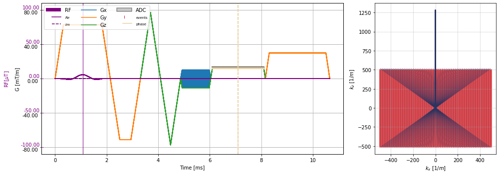
Rotate gradients to XYZ and plot

rot_matrix = cmrseq.utils.get_rotation_matrix(slice_normal, readout_direction, target_orientation='xyz')

for seq in sequence_list:
    seq.rotate_gradients(rot_matrix)

_, k_adc, t_adc = sequence_list[0].calculate_kspace()


plt.close("all")
f, (a1, a2) = plt.subplots(1, 2, figsize=(14, 5), gridspec_kw={'width_ratios': [5, 2]})
cmrseq.plotting.plot_sequence(sequence_list[0], axes=a1, adc_yoffset=15.7)
for s in sequence_list[1:]:
    cmrseq.plotting.plot_sequence(s, axes=[f.axes[-1], a1, a1, a1], format_axes=False, adc_yoffset=15.7)

for s in sequence_list:
    cmrseq.plotting.plot_kspace_2d(s, ax=a2, k_axes=[0, 2])
f.tight_layout()

Set up Phantom

Load mesh

# Load Aorta Example.
mesh = pyvista.read("../example_resources/steady_stenosis.vtk")

# The velocity [m/s] is stored in the mesh as U1. In cmrsim all definitions are done in [ms] therefore
# We add the velocity field as scaled data to the mesh
mesh["velocity"] = Quantity(mesh["U"], "m/s").m_as("m/ms")

# To match the usual geometry (Head <-> Foot along z-axis) flip the axes of the mesh
mesh.points = mesh.points[:,[2,1,0]]
mesh.points[:, 1:] *= -1
mesh["velocity"] = mesh["velocity"][:,[2,1,0]]
mesh["velocity"][:, 1:] *= -1
global_mesh_offset = [0.0, 0.0, 0.1]
mesh.translate(global_mesh_offset, inplace=True)
mesh = mesh.cell_data_to_point_data()

# clip to restricted length to reduce mesh-size
mesh.clip(normal='z', origin=[0., 0., 0.11], inplace=True)
mesh.clip(normal='-z', origin=[0., 0., -0.10], inplace=True)

Header	Data Arrays
UnstructuredGrid Information N Cells 877450 N Points 897024 X Bounds -1.500e-02, 1.500e-02 Y Bounds -1.500e-02, 1.500e-02 Z Bounds -1.000e-01, 1.000e-01 N Arrays 2	Name Field Type N Comp Min Max U Points float64 3 -7.556e-02 4.969e-01 velocity Points float64 3 -4.969e-04 8.997e-05

Instantiate Refilling dataset

# Setup flow dataset with seeding mesh information
particle_creation_fncs = {"magnetization": part_factory.norm_magnetization(),
                          "T1": part_factory.uniform(default_value=250.),
                          "T2": part_factory.uniform(default_value=50.),
                          "M0": part_factory.uniform(default_value=1/seeding_particle_density)}

dataset = cmrsim.datasets.RefillingFlowDataset(mesh,
                                               particle_creation_callables=particle_creation_fncs,
                                               slice_position=seeding_slice_position.m_as("m"),
                                               slice_normal=seeding_slice_normal,
                                               slice_thickness=seeding_slice_thickness.m_as("m"),
                                               slice_bounding_box=seeding_slice_bb.m_as("m"),
                                               seeding_vol_spacing=seeding_pixel_spacing,
                                               lookup_map_spacing=lookup_map_spacing,
                                               field_list=[("velocity", 3)])

lookup_table_3d, map_dimensions = dataset.get_lookup_table()
trajectory_module = cmrsim.datasets.FlowTrajectory(velocity_field=lookup_table_3d.astype(np.float32),
                                                   map_dimensions=map_dimensions.astype(np.float32),
                                                   additional_dimension_mapping=dataset.field_list[1:],
                                                   device='GPU')

Updated Mesh
Updated Slice Position

Visualize

Legend: - Red box: Slice selective excitation - White Plane: Imaging plane - Orange Box: Re-seeding volume

pyvista.close_all()
pyvista.set_jupyter_backend('panel')
pyvista.start_xvfb()
plotter = pyvista.Plotter(notebook=True, window_size=(1000, 500), shape=(1, 2))

# Plot axes at origin
origin_arrows = [pyvista.Arrow(start=(0., 0., 0.), direction=direction, tip_length=0.1, tip_radius=0.025,
                               tip_resolution=10, shaft_radius=0.005, shaft_resolution=10, scale=0.1)
                 for direction in [(1., 0., 0.), (0., 1., 0.), (0., 0., 1.)]]
plotter.add_mesh(origin_arrows[0], color="blue", label="x")
plotter.add_mesh(origin_arrows[1], color="green", label="y")
plotter.add_mesh(origin_arrows[2], color="red", label="z")

# Plot input mesh
plotter.add_mesh(mesh, scalars="velocity", opacity=0.6, colormap="seismic")

# Plot slice selective RF
_scale = 0.1
rf_mesh = pyvista.Box(bounds=(-_scale, _scale, -_scale, _scale, -slice_thickness.m_as("m")/2, slice_thickness.m_as("m")/2))
rf_mesh.points = cmrseq.utils.mps_to_xyz(rf_mesh.points[np.newaxis], slice_normal=slice_normal, readout_direction=np.array([1., 0., 0.]))[0]
rf_mesh.translate(slice_position, inplace=True)
plotter.add_mesh(rf_mesh, opacity=0.1, show_edges=True, color="red")

# Plot projection plane of the cartesian image slice with M-S directions
image_slice_mesh = pyvista.Box(bounds=(-fov[0].m_as("m")/2, fov[0].m_as("m")/2, -fov[1].m_as("m")/2, fov[1].m_as("m")/2, 0, 0))
image_slice_mesh.points = cmrseq.utils.xyz_to_mps(image_slice_mesh.points[np.newaxis], slice_normal=slice_normal, readout_direction=readout_direction)[0]
readout_glyph = pyvista.Arrow(start=slice_position.m_as("m"), direction=readout_direction, tip_length=0.1, tip_radius=0.025,
                               tip_resolution=10, shaft_radius=0.01, shaft_resolution=10, scale=0.05)
slice_selection_glyph = pyvista.Arrow(start=slice_position.m_as("m"), direction=slice_normal, tip_length=0.1, tip_radius=0.025,
                               tip_resolution=10, shaft_radius=0.01, shaft_resolution=10, scale=0.05)

plotter.add_mesh(image_slice_mesh, opacity=0.3, show_edges=True)
plotter.add_mesh(readout_glyph, color="black")
plotter.add_mesh(slice_selection_glyph, color="black")

# Plot the slice in which the re-seeding is performed
plotter.add_mesh(dataset.gridded_seeding_volume, color="orange", opacity=1, show_edges=False)

# Plot seeded particles
plotter.subplot(0, 1)
initial_position, _ = dataset.initial_filling(particle_density=8, slice_dictionary=dict(slice_normal=seeding_slice_normal,
                                              slice_position=seeding_slice_position.m_as("m"), slice_thickness=seeding_slice_thickness.m_as("m")))

pos, additional_fields = trajectory_module(initial_position, dt=0.01, n_steps=100, return_velocities=True)
plotter.add_mesh(pyvista.PolyData(initial_position), scalars=additional_fields[-1]["velocity"], cmap="seismic")
plotter.show()

Simulation

After each TR, the RefillingDataset re-seeds particles to compensate the outflow.

time_rf, rf_grid, grad_grid, adc_on_grid = [np.stack(v) for v in cmrseq.utils.grid_sequence_list(sequence_list, force_uniform_grid=False)]
print("Input shapes for Bloch Module:\n  ", "\n   ".join([f"{time_rf.shape=}", f"{rf_grid.shape=}",
                                                          f"{grad_grid.shape=}", f"{adc_on_grid.shape=}"]))

module = cmrsim.bloch.GeneralBlochOperator(name="rf", gamma=system_specs.gamma_rad.m_as("rad/mT/ms"),
                                           time_grid=time_rf[0], gradient_waveforms=grad_grid,
                                           rf_waveforms=rf_grid, adc_events=adc_on_grid, device="GPU:0")

initial_position, properties = dataset.initial_filling(particle_density=seeding_particle_density,
                                                       slice_dictionary=dict(slice_normal=seeding_slice_normal,
                                                                             slice_position=seeding_slice_position.m_as("m"),
                                                                             slice_thickness=seeding_slice_thickness.m_as("m")))
print(initial_position.shape, time_rf.shape)
n_samples = tf.shape(module.time_signal_acc[0])[0]
n_repetitions = tf.shape(module.gradient_waveforms)[0]

r = initial_position
for rep_idx in tqdm(range(time_rf.shape[0])):
    m = properties.pop("magnetization")
    m, r = module(trajectory_module=trajectory_module, initial_position=r, magnetization=m,
                  repetition_index=rep_idx, run_parallel=False, **properties)
    properties["magnetization"] = m.numpy()
    r, properties, _ = dataset(particle_density=seeding_particle_density, residual_particle_pos=r.numpy(),
                               particle_properties=properties, distance_tolerance=0.2, reseed_threshold=0.5)

Reconstruct Image

time_signal = tf.stack(module.time_signal_acc, axis=0).numpy().reshape(matrix_size[::-1])
centered_projection = tf.signal.fft(time_signal).numpy()
centered_k_space = tf.signal.fft(centered_projection).numpy()
image = tf.signal.fftshift(tf.signal.ifft2d(tf.roll(tf.signal.ifftshift(centered_k_space, axes=(0, 1)),  -1, axis=1)), axes=(0, 1)).numpy()
time_per_seg = t_adc - t_adc[matrix_size[0]//2+1]
freq_per_seg = np.fft.fftfreq(n=time_per_seg.shape[0], d=time_per_seg[1]-time_per_seg[0])

print(time_signal.shape, centered_projection.shape, time_per_seg.shape, freq_per_seg.shape, image.shape)

(61, 301) (61, 301) (301,) (301,) (61, 301)

Plot Results

Plot 2D representation of specific single line acquisitions

If the configured adc only acquires the exact k-space locations the acquired time signal equals the k-space line

# Plot 2D Lines
fig, axes = plt.subplots(1, 4, figsize=(18, 3))
[a.grid(True) for a in axes]
[a.set_title(t) for a, t in zip(axes, ["temporal signal", "spectrum", "k-space line", "spatial projection"])]
[a.legend(["real", "Imaginary"]) for a in axes]
for ky in range(0, time_signal.shape[0], 10):
    axes[0].plot(time_per_seg, np.real(time_signal[ky]), color="C0", linestyle="-", alpha=0.7)
    axes[0].plot(time_per_seg, np.imag(time_signal[ky]), color="C1", linestyle="-", alpha=0.7)
    axes[1].plot(freq_per_seg, np.real(centered_projection[ky]), color="C0", linestyle="-", alpha=0.7)
    axes[1].plot(freq_per_seg, np.imag(centered_projection[ky]), color="C1", linestyle="-", alpha=0.7)
    axes[2].plot(np.arange(freq_per_seg.shape[0]), np.real(centered_k_space[ky]), color="C0", linestyle="-", alpha=0.7)
    axes[2].plot(np.arange(freq_per_seg.shape[0]), np.imag(centered_k_space[ky]), color="C1", linestyle="-", alpha=0.7)
    axes[3].plot(np.arange(freq_per_seg.shape[0]), np.real(image[ky]), color="C0", linestyle="-", alpha=0.7)
    axes[3].plot(np.arange(freq_per_seg.shape[0]), np.imag(image[ky]), color="C1", linestyle="-", alpha=0.7)
fig.tight_layout()

Plot 3D representation of simulation results

If the configured adc only acquires the exact k-space locations the acquired time signal equals the k-space line

# Plot all PE-lines in 3D
plt.close("all")
from mpl_toolkits.mplot3d.axes3d import Axes3D
fig, axes = plt.subplots(1, 4, subplot_kw={'projection': '3d'}, figsize=(18, 4))
[a.set_title(t) for a, t in zip(axes, ["temporal signal", "spectrum", "k-space line", "spatial projection"])]

for ky in range(time_signal.shape[0]):
    axes[0].plot(time_per_seg, np.ones_like(time_signal[ky].real) * ky, np.abs(time_signal[ky]), color="C0", linestyle="-", alpha=0.7)
    axes[1].plot(freq_per_seg, np.ones_like(centered_projection[ky].real) * ky, np.abs(centered_projection[ky]), color="C0", linestyle="-", alpha=0.7)
    axes[2].plot(np.arange(freq_per_seg.shape[0]), np.ones_like(centered_k_space[ky].real) * ky, np.abs(centered_k_space[ky]), color="C0", linestyle="-", alpha=0.7)
    axes[3].plot(np.arange(freq_per_seg.shape[0]), np.ones_like(image[ky].real) * ky, np.abs(image[ky]), color="C0", linestyle="-", alpha=0.7)
fig.tight_layout()

Plot Image

# Show images
fig, axes = plt.subplots(3, 1, figsize=(18, 11))

kspace_plot = axes[0].imshow(np.log(np.abs(np.squeeze(centered_k_space))), cmap="gray")
fig.colorbar(kspace_plot, ax=axes[0], fraction=0.015, pad=0.005)
abs_plot = axes[1].imshow(np.abs(np.squeeze(image)), cmap="gray")
fig.colorbar(abs_plot, ax=axes[1], fraction=0.015, pad=0.005)
phase_plot = axes[2].imshow(np.angle(np.squeeze(image)), cmap="twilight", vmin=-np.pi, vmax=np.pi)
fig.colorbar(phase_plot, ax=axes[2], fraction=0.015, pad=0.005)
[(_.set_yticks([]), _.set_xticks([])) for _ in axes]
[_.set_ylabel(t, fontsize=20) for _, t in zip(axes, ["k-space", "Magnitude", "Phase"])]
fig.tight_layout()