Basics of performing Analytic Simulations#

This notebooks aims to show only the basic concepts of analytic simulations inside the cmrsim frame work. The incorporation of motion is shown in the next notebook.

It is subdivided into the following subsections:

- Define the simulation - Define a digital phantom - Run the simulation - Auxiliary functions to save the simulation config

Imports#

For multi GPU environments, here the usage is limited to the first visibible device. In case no GPU is available CPU is used by default.

In case cmrsim is not installed in the virtual environment the repository root is added to the python path.

[1]:

import sys
sys.path.insert(0, "../../")  # if cmrsim-repository was cloned -> import from there
sys.path.append("../")  # to import local_functions

import base64
from IPython.display import display, HTML, clear_output

import tensorflow as tf
physical_devices = tf.config.list_physical_devices('GPU')
if physical_devices:
    print("Available GPUS: \n\t", "\n\t".join([str(_) for _ in physical_devices]))
    tf.config.experimental.set_visible_devices(physical_devices[0], 'GPU')
    tf.config.experimental.set_memory_growth(physical_devices[0], True)

from collections import OrderedDict
import numpy as np
import math
from pint import Quantity
import pyvista

import matplotlib.pyplot as plt
%matplotlib inline

import cmrsim
import local_functions
clear_output()

Define the simulation#

As described in the readme and the documentation of the SimulationBase-class, there is the convenient way of subclassing the abstract Base-class. All subclasses need to implement the the _build method, where the composition of building blocks is performed. As the simulation parameters are defined as tf.Variables their values are easily modifyable at any time, even with graph execution.

The _build member-function must return a triple containing an instance of a subclassed EncodingBase module, a CompositeSignalModel (composing all signal operator building blocks) and an instance of a ReconBase module. If the simulation is meant to return the k-space signal, the third entry of the returned triple can be set to None.

The following ExampleSimulation is setup as a single shot (EPI) spin-echo, considering the T2* effects (TE-t, TE+t) with a simple inverse FFT as reconstruction.

[2]:

from typing import Tuple
class ExampleSimulation(cmrsim.analytic.AnalyticSimulation):
    def build(self, matrix_size: Tuple[int, int] = (80, 100),
              field_of_view: Tuple[float, float] = (0.25, 0.3)):
        n_kx, n_ky = matrix_size

        # Encoding definition / To enable result comparisons, the noise is set to 0 here
        encoding_module = cmrsim.analytic.encoding.EPI(field_of_view=field_of_view, sampling_matrix_size=matrix_size,
                                                       read_out_duration=0.4, blip_duration=0.01, k_space_segments=1,
                                                       absolute_noise_std=0.)
        # Signal module construction
        spinecho_module = cmrsim.analytic.contrast.SpinEcho(echo_time=50, repetition_time=10000, expand_repetitions=True)

        centered_times = tf.abs(encoding_module.get_sampling_times() - tf.reduce_max(encoding_module.get_sampling_times()) / 2)
        t2_star_module =  cmrsim.analytic.contrast.t2_star.StaticT2starDecay(centered_times, expand_repetitions=False)

        # Forward model composition
        forward_model = cmrsim.analytic.CompositeSignalModel(spinecho_module, t2_star_module)

        # Reconstruction
        recon_module = cmrsim.reconstruction.Cartesian2D(sample_matrix_size=(n_kx, n_ky), padding=None)
        return forward_model, encoding_module, recon_module

To run the simulation, a Simulator-object needs to be instantiated.

[3]:

field_of_view = Quantity((0.25, 0.3), "m")
matrix_size = (80, 100)
simulator = ExampleSimulation(name='simulation_example', build_kwargs=dict(matrix_size=matrix_size, field_of_view=field_of_view.m_as("m").tolist()))

/tmp/ipykernel_37976/2672367390.py:8: DeprecationWarning: Call to deprecated class EPI. (Consider using the cmrsim.analytic.encoding.GenericEncoding class incombination with a cmrseq.sequence definition)
  encoding_module = cmrsim.analytic.encoding.EPI(field_of_view=field_of_view, sampling_matrix_size=matrix_size,

Now display what the requirements for the digital phantoms are, i.e. which physical properties must each material point have assigned:

[4]:

simulator.forward_model.required_quantities, simulator.get_k_space_shape()

[4]:

(('M0', 'T1', 'T2', 'T2star'),
 <tf.Tensor: shape=(2,), dtype=int32, numpy=array([   1, 8000], dtype=int32)>)

Define a digital phantom#

In the following cell, a 2D object is constructed by loading a semantic mask (labels are integers) from the XCAT phantom.

The coordinates are assumed to lie on a regular-grid, therefore the utility of cmrsim.utils.coordinates is an easy way to calculate them.

As described in the README, the digital phantom is defined as OrderedDictionary of numpy arrays, where the keys are named after the entries of the required quantities. Furthermore, the assign_to_numerical_label_map is used to assign values according to the semantic label of the input map.

[5]:

phantom_mesh = local_functions.create_cylinder_phantom()
clear_output()
phantom_mesh

[5]:

Header

Data Arrays

UnstructuredGrid	Information
N Cells	96456
N Points	130204
X Bounds	-1.000e-01, 9.900e-02
Y Bounds	-1.000e-01, 9.900e-02
Z Bounds	-5.000e-03, 2.500e-03
N Arrays	5

Name	Field	Type	N Comp	Min	Max
class	Points	int32	1	-1.000e+00	3.000e+00
M0	Points	float64	1	0.000e+00	9.000e-01
T1	Points	float64	1	0.000e+00	1.000e+03
T2	Points	float64	1	0.000e+00	2.500e+02
T2star	Points	float64	1	0.000e+00	5.000e+01

[6]:

pyvista.close_all()
pyvista.start_xvfb()
plotter = pyvista.Plotter(window_size=(1600, 300), off_screen=True, shape=(1, 4))
for idx, sc in enumerate(["class", "M0", "T1", "T2"]):
    plotter.subplot(0, idx)
    plotter.add_mesh(phantom_mesh.copy(), scalars=sc)
    local_functions.add_custom_axes(plotter, scale=0.2)
    box = local_functions.transformed_box(reference_basis=np.eye(3, 3), slice_normal=np.array([0., 0., 1.]), readout_direction=np.array([1., 0., 0.]),
                                          slice_position=Quantity([0., 0., 0.], "m"), extend=Quantity([*field_of_view.m_as("m"), 0.01], "m"))
    plotter.add_mesh(box, color="white", opacity=0.5)
plotter.screenshot("phantom_example.png")
b64 = base64.b64encode(open("phantom_example.png",'rb').read()).decode('ascii')
display(HTML(f'<img src="data:image/gif;base64,{b64}" />'))

/scratch/jweine/cmrsim/notebooks/analytic_simulation/../local_functions.py:43: UserWarning: Optimal rotation is not uniquely or poorly defined for the given sets of vectors.
  rot, _ = Rotation.align_vectors(reference_basis, new_basis)

To pass the phantom into the simulator, the a dictionary is used to instantiate a costum tf.data.Dataset implemented in the BaseDataset class. The dictionary contains numpy arrays corresponding to the required quantities listed above.

[7]:

phantom_dict = dict(
    M0=phantom_mesh["M0"].astype(np.complex64),
    T1=phantom_mesh["T1"].astype(np.float32),
    T2=phantom_mesh["T2"].astype(np.float32),
    T2star=phantom_mesh["T2star"].astype(np.float32),
    r_vectors=phantom_mesh.points.astype(np.float32))

print("Phantom Definition: \t" , [f"{k}:{v.shape}" for k, v in phantom_dict.items()])
dataset = cmrsim.datasets.AnalyticDataset(phantom_dict, filter_inputs=True, expand_dimension=True)

Phantom Definition:      ['M0:(130204,)', 'T1:(130204,)', 'T2:(130204,)', 'T2star:(130204,)', 'r_vectors:(130204, 3)']

Run the simulation#

To start the simulation, use the __call__ function of the simulator instance {() - operator}.

[9]:

%time simulation_result = simulator(dataset, voxel_batch_size=10000)
simulation_result.shape

2022-12-22 09:37:15.349310: I tensorflow/core/grappler/optimizers/data/replicate_on_split.cc:32] Running replicate on split optimization

WARNING:tensorflow:From /scratch/jweine/conda/envs/tf29_pyvista/lib/python3.9/site-packages/tensorflow/python/autograph/pyct/static_analysis/liveness.py:83: Analyzer.lamba_check (from tensorflow.python.autograph.pyct.static_analysis.liveness) is deprecated and will be removed after 2023-09-23.
Instructions for updating:
Lambda fuctions will be no more assumed to be used in the statement where they are used, or at least in the same block. https://github.com/tensorflow/tensorflow/issues/56089
Run Simulation:         |XXXXXXXXXXXXXXX|127548/127548  |XXXXXXXXXXXXXXX|1/1 CPU times: user 4 s, sys: 705 ms, total: 4.71 s
Wall time: 4.68 s

[9]:

TensorShape([1, 100, 80])

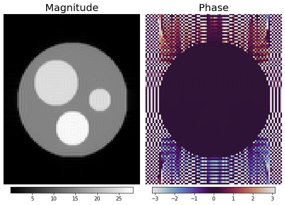
[10]:

import ipywidgets as widgets

f, a = plt.subplots(1, 2, figsize=(8, 6))
magnitude_image = np.squeeze(np.abs(simulation_result))
phase_image = np.squeeze(np.angle(simulation_result))
# img0 = a[0].imshow(phantom_reference_map, origin="lower")
img1 = a[0].imshow(magnitude_image, cmap="gray")
img2 = a[1].imshow(phase_image, cmap="twilight")
[plt.colorbar(im, ax=ax, location="bottom", pad=0.01, shrink=0.9) for im, ax in zip([img1, img2], a)]
[_.axis("off") for _ in a.flatten()]
[_.set_title(t, fontsize=20) for _, t in zip(a, ("Magnitude", "Phase"))]
f.tight_layout()

../../_images/example_gallery_analytic_simulation_1_basic_functionality_16_0.png

Auxilliary functions#

1. Saving and Loading#

The next cell shows how the simulation with all its configurations can be saved as tf.train.Checkpoint, and afterwards be restored from the checkpoint by calling the classmethod SimulationBase.from_checkpoint(...). To ensure that the parameters are equal, the simulation is redone and the results are compared.

[11]:

import os

# Specify saving path
chkpt = './model_checkpoints/example_checkpoint'
os.makedirs(os.path.dirname(chkpt), exist_ok=True)

# Save simulation to checkpoint and delete old instance
simulator.save(checkpoint_path=chkpt)
del simulator

# construct new intance from checkpoint
new_simulator = ExampleSimulation.from_checkpoint(chkpt)

/tmp/ipykernel_37976/2672367390.py:8: DeprecationWarning: Call to deprecated class EPI. (Consider using the cmrsim.analytic.encoding.GenericEncoding class incombination with a cmrseq.sequence definition)
  encoding_module = cmrsim.analytic.encoding.EPI(field_of_view=field_of_view, sampling_matrix_size=matrix_size,

[13]:

%time simulation_load_result = new_simulator(dataset, voxel_batch_size=5000)

print("If this is equal to zero, the simulated results are identical:\n\t Difference of simulated k-space ->",
      tf.reduce_sum(simulation_result - simulation_load_result))

2022-12-22 09:37:58.241793: I tensorflow/core/grappler/optimizers/data/replicate_on_split.cc:32] Running replicate on split optimization

Run Simulation:         |XXXXXXXXXXXXXXX|127548/127548  |XXXXXXXXXXXXXXX|1/1 CPU times: user 2.84 s, sys: 283 ms, total: 3.12 s
Wall time: 2.67 s
If this is equal to zero, the simulated results are identical:
         Difference of simulated k-space -> tf.Tensor((0.005216048-0.00024144002j), shape=(), dtype=complex64)

2. Manipulate Parameters#

After instantitation of simulator instances, the variables contained in the submodules can be changed by directly accesing the tf.Variable.assign() method. To show if the results differ after setting different Echo-Times the simulated images are compared again:

[14]:

new_simulator.forward_model.spin_echo.TE.assign([10,])  # in milliseconds
%time n = new_simulator(dataset, voxel_batch_size=5000)
print('Mean absolute difference for different TE:', tf.reduce_mean(tf.abs(simulation_load_result - n)))

new_simulator.forward_model.spin_echo.TE.assign([50,]) # in milliseconds
%time n = new_simulator(dataset, voxel_batch_size=5000)
print('Mean absolute difference for same TE:', tf.reduce_mean(tf.abs(simulation_load_result - n)))

Run Simulation:         |X--------------|10000/127548   |XXXXXXXXXXXXXXX|1/1

2022-12-22 09:38:17.803139: I tensorflow/core/grappler/optimizers/data/replicate_on_split.cc:32] Running replicate on split optimization

Run Simulation:         |XXXXXXXXXXXXXXX|127548/127548  |XXXXXXXXXXXXXXX|1/1 CPU times: user 1.53 s, sys: 280 ms, total: 1.81 s
Wall time: 1.39 s
Mean absolute difference for different TE: tf.Tensor(1.5230018, shape=(), dtype=float32)
Run Simulation:         |X--------------|15000/127548   |XXXXXXXXXXXXXXX|1/1

2022-12-22 09:38:19.192124: I tensorflow/core/grappler/optimizers/data/replicate_on_split.cc:32] Running replicate on split optimization

Run Simulation:         |XXXXXXXXXXXXXXX|127548/127548  |XXXXXXXXXXXXXXX|1/1 CPU times: user 1.44 s, sys: 309 ms, total: 1.75 s
Wall time: 1.34 s
Mean absolute difference for same TE: tf.Tensor(0.0, shape=(), dtype=float32)

3. Display summary as JSON#

The SimulationBase class includes a functionality to create a report of the simulation configuration (aka submodule Variables) as dictionary. This dictionary can be used to generate a JSON string

[15]:

import json
from IPython.display import JSON

summary_dict = new_simulator.configuration_summary
JSON(json.dumps(summary_dict))

/scratch/jweine/conda/envs/tf29_pyvista/lib/python3.9/site-packages/IPython/core/display.py:606: UserWarning: JSON expects JSONable dict or list, not JSON strings
  warnings.warn("JSON expects JSONable dict or list, not JSON strings")

[15]:

<IPython.core.display.JSON object>