Bloch-Simulation of PRESS in a moving heart#
Content: 1. Load pre-defined contracting cardiac mesh 2. Instatiate Trajectory module 2. Define sequence 3. Run CMRsim simulation 4. Analyze Data
Import & Definitions#
[1]:
## Install the cmr_rnd_diffusion package (https://gitlab.ethz.ch/jweine/cmr-random-diffmaps/-/packages)
# !pip install cmr-rnd-diffusion==1.5 --extra-index-url https://__token__:????????@gitlab.ethz.ch/api/v4/projects/29882/packages/pypi/simpl
[2]:
import os
import math
from typing import List, Union, Tuple, Sequence
import sys

import pyvista
import numpy as np
from tqdm.notebook import tqdm
import matplotlib.pyplot as plt
from pint import Quantity
from scipy.optimize import curve_fit

import tensorflow as tf
gpu = tf.config.get_visible_devices("GPU")[0]
tf.config.set_visible_devices(gpu, device_type="GPU")
tf.config.experimental.set_memory_growth(gpu, True)

import cmr_rnd_diffusion
sys.path.insert(0, "../../")
sys.path.insert(0, "../../../cmrseq/")
import cmrsim
import cmrseq
C:\Users\Jonat\anaconda3\envs\tf29_pyvista\lib\site-packages\cdtipy\reconstruction.py:11: UserWarning: No matlab installation found!
  warnings.warn("No matlab installation found!")
C:\Users\Jonat\anaconda3\envs\tf29_pyvista\lib\site-packages\cdtipy\registration.py:10: UserWarning: No matlab installation found!
  warnings.warn("No matlab installation found!")
Next cell only defines the pyvista plotting settings of my personal choice :)
[3]:
custom_theme = pyvista.themes.DefaultTheme()
custom_theme.background = 'white'
custom_theme.font.family = 'times'
custom_theme.font.color = 'black'
custom_theme.outline_color = "white"
custom_theme.edge_color = 'grey'
custom_theme.transparent_background = True
Load mesh#
Load full mesh
Animate the full mesh
Select a thick slab
Instantiate a trajectory module for simulation
Load full Mesh#
[4]:
fn = "../example_resources/refined_mesh_(23,161,150).vtk"
mesh_numbers = [int(s) for s in os.path.basename(fn).replace("refined_mesh_(", "").replace(").vtk", "").split(",")]
refined_mod = cmrsim.datasets.CardiacMeshDataset.from_single_vtk(fn, time_precision_ms=3, mesh_numbers=mesh_numbers)

# If you uncomment the following line, you will get a lengthy summary of data contained inside the vtk mesh:
# refined_mod.mesh
To produce a fancy looking animation of the mesh execute the next cell. As mesh-fields, the displacements for multiple times (compare with the summary above).
Animate#
[5]:
pyvista.close_all()
pyvista.start_xvfb()
plotter = pyvista.Plotter(off_screen=True, theme=custom_theme, window_size=(800, 800))

refined_mod.render_input_animation(filename="fancy_input_animation_test.gif", plotter=plotter,
                                   start=Quantity(0., "ms"), end=Quantity(280, "ms"))
Select thick slab#
[6]:
# Select slice according to the following slice parameters:
slice_dict = dict(slice_thickness=Quantity(10, "mm"),
                  slice_normal=np.array((0., 0., 1.)),
                  slice_position=Quantity([0, 0, -3], "cm"),
                  reference_time=Quantity(105, "ms"))

slice_mesh = refined_mod.select_slice(**slice_dict)
slice_mod =  cmrsim.datasets.MeshDataset(slice_mesh, refined_mod.timing)

# Now get actual time / positional values for all points contained in the mesh:
t, r = slice_mod.get_trajectories(start=slice_dict["reference_time"],
                                  end=Quantity(slice_mod.timing[-1], "ms"))

print(f"Temporal reference grid: {t.shape}[{t.units}]",
      f"Positions at reference times: {r.shape} [{r.units}]")
Temporal reference grid: (45,)[millisecond] Positions at reference times: (60759, 45, 3) [meter]
Fit Taylor expansion for each particle#
This trajectory module can be directly handed to the simulation below
[7]:
trajectory_mod = cmrsim.trajectory.TaylorTrajectoryN(order=6, time_grid=t-t[0],
                                                     particle_trajectories=r)
The next cell is only to show you how the trajectory module can be used:
[8]:
# Define new time-grid
# new_tgrid = tf.range(0, 200, 2, dtype=tf.float32)

# # Call the module to get all new positions. Note, the second returned dict is useless in our case.
# new_positions, _ = trajectory_mod(new_tgrid)

# print(f"Time grid: {new_tgrid.shape},  Positions: {new_positions.shape}")

# # Animate the mesh motion with new positions:
# new_positions = np.array(new_positions)  # necessary for plotting below
# cp_mesh = slice_mod.mesh.copy()
# pyvista.close_all()
# pyvista.start_xvfb()
# plotter = pyvista.Plotter(off_screen=True, window_size=(800, 800))
# plotter.add_mesh(cp_mesh)
# plotter.open_gif(f"TaylorTrajectory.gif")
# for step in tqdm(range(0, len(new_tgrid)), desc="Redering Mesh-Animation"):
#     text_actor = plotter.add_text(f"{new_tgrid[step]: 1.0f} ms", position='upper_right', color='grey',
#                                   shadow=False, font_size=26, render=False)
#     plotter.update_coordinates(new_positions[:, step], mesh=cp_mesh, render=False)
#     plotter.render()
#     plotter.write_frame()
#     plotter.remove_actor(text_actor)
# plotter.close()
Define Sequence#
Set system limits
Instantiate sequence with fancy gradients
Grid sequence for simulation
[9]:
# The raster times here, directly influence the bloch-simulation step-width
system_specs = cmrseq.SystemSpec(gamma=Quantity(42.576, 'MHz / T'),
                                 max_grad=Quantity(40, "mT/m"),
                                 max_slew=Quantity(80, "mT/m/ms"),
                                 grad_raster_time=Quantity(10, "us"),
                                 rf_raster_time=Quantity(10, "us")
                                )
This of course is only a placeholder:
[10]:
# Reuse slice definition from above:
slice_dict = dict(slice_thickness=Quantity(10, "mm"),
                  slice_normal=np.array((0., 0., 1.)),
                  slice_position=Quantity([0, 0, -3], "cm"),
                  reference_time=Quantity(105, "ms"))


seq = cmrseq.seqdefs.excitation.slice_selective_sinc_pulse(system_specs,
                                                          slice_normal=np.array((0., 0., 1.)),
                                                          slice_position_offset=Quantity(0, "cm"),
                                                          slice_thickness=Quantity(1000, "mm"),
                                                          flip_angle=Quantity(90, "degree"),
                                                          pulse_duration=Quantity(2, "ms"),
                                                          time_bandwidth_product=6)
readout = cmrseq.seqdefs.readout.gre_cartesian_line(system_specs, num_samples=100,
                                                    k_readout=Quantity(10, "1/m"),
                                                    k_phase=Quantity(0, "1/m"),
                                                    adc_duration=Quantity(4, "ms"))
seq.append(readout)
C:\Users\Jonat\anaconda3\envs\tf29_pyvista\lib\site-packages\pint\quantity.py:1313: RuntimeWarning: invalid value encountered in double_scalars
  magnitude = magnitude_op(new_self._magnitude, other._magnitude)
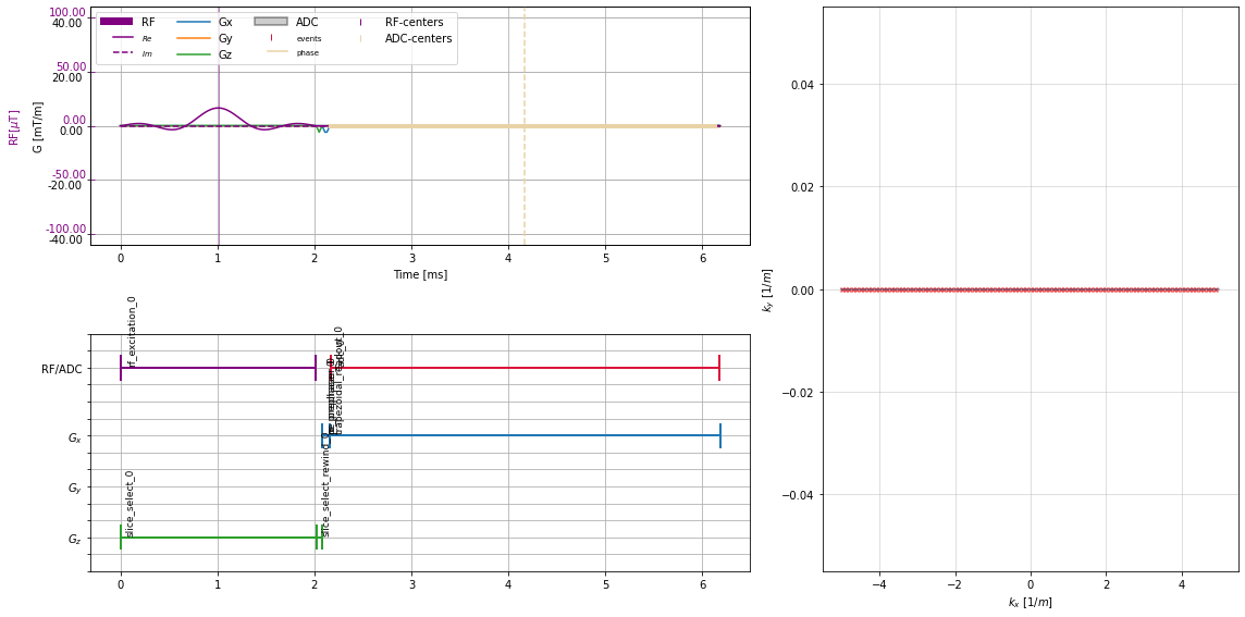
Plot the sequence#
[11]:
plt.close("all")
fig = plt.figure(figsize=(16, 8))
axes = fig.subplot_mosaic("AAABB;CCCBB")
cmrseq.plotting.plot_sequence(seq, axes=axes["A"], format_axes=True);
cmrseq.plotting.plot_block_names(seq, axis=axes["C"]);
cmrseq.plotting.plot_kspace_2d(seq, ax=axes["B"]);
fig.tight_layout()
Grid sequence#
[12]:
time_raster, rf_raster, wf_raster, adc_raster = grid_out = [np.stack(v) for v in cmrseq.utils.grid_sequence_list(sequence_list=[seq, ], force_uniform_grid=False)]
print("Waveforms on raster: \n\t", "\n\t".join([f"{name:<15}: {v.shape}  | {v.dtype}"
                                                for name, v in zip("time_raster,rf_raster,wf_raster,adc_raster".split(","), grid_out)]))
Waveforms on raster:
         time_raster    : (1, 619)  | float64
        rf_raster      : (1, 619)  | complex128
        wf_raster      : (1, 619, 3)  | float64
        adc_raster     : (1, 619, 2)  | float64
Bloch - Simulation#
Assign physical properties
Construct Bloch operator
Run simulation
[18]:
from cmrsim.utils import particle_properties as part_factory

initial_positions, _ = trajectory_mod(tf.constant([0.,], dtype=tf.float32))  # is already in meter
n_particles = initial_positions.shape[0]

phantom_dict = {
    "M0":  tf.ones(n_particles),         # Used for scaling. If constant --> all particle are weighted the same for summation
    "T1":   tf.random.normal(shape=(n_particles,), mean=1000, stddev=100),  # in millisecond
    "T2":  tf.random.normal(shape=(n_particles, ), mean=200, stddev=20),   # in millisecond
    "off_res": tf.random.normal(shape=(n_particles, 1), mean=0, stddev=3),
    "magnetization": part_factory.norm_magnetization()(n_particles),   # constructs complex magnetization vector for each particle
    "initial_position": tf.reshape(initial_positions, [-1, 3])
}

dataset = cmrsim.datasets.BlochDataset(phantom_dict, filter_inputs=False)

t, r = slice_mod.get_trajectories(start=slice_dict["reference_time"],
                                  end=Quantity(slice_mod.timing[-1], "ms"))
trajectory_mod = cmrsim.trajectory.TaylorTrajectoryN(order=6, time_grid=t-t[0],
                                                     particle_trajectories=r, batch_size=int(1e6))
rout, _ = trajectory_mod.increment_particles(None, 0.01)
rout;
[19]:
submods = [cmrsim.bloch.submodules.OffResonance(system_specs.gamma_rad.m_as("rad/mT/ms"))]

bloch_module = cmrsim.bloch.GeneralBlochOperator(name="testmodule",
                                                gamma=system_specs.gamma_rad.m_as("rad/mT/ms"),
                                                time_grid=time_raster[0],
                                                gradient_waveforms=wf_raster,
                                                rf_waveforms=rf_raster,
                                                adc_events=adc_raster,
                                                submodules=submods,
                                                device="GPU:0")
[20]:
# tf.config.run_functions_eagerly(True)
tf.config.run_functions_eagerly(False)
bloch_module.reset()
trajectory_mod.current_time_ms.assign(0.)
for bidx, batch in tqdm(enumerate(dataset(batchsize=int(1e6)))):
    trajectory_mod.current_batch_idx.assign(bidx)
    _ = bloch_module(trajectory_module=trajectory_mod, **batch)
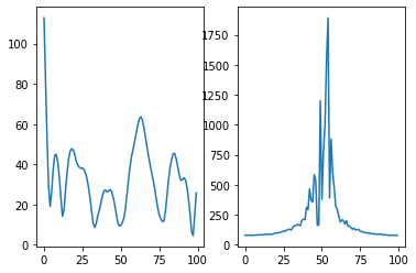
Analyze Data#
[21]:
signal = bloch_module.time_signal_acc[0].numpy()
spectrum = np.fft.fftshift(np.fft.fft(signal))
[22]:
fig, axis = plt.subplots(1, 2)
axis[0].plot(np.abs(signal));
axis[1].plot(np.abs(spectrum));
[ ]: