Multiple Coils: Using the ParallelReceiveBlochOperator#
In this notebook, the incorporation of coil-sensitivities into Bloch-simulation is highlighted. To do so, first a 3-dimensional coil-sensitivity map is computed assuming an ideal Birdcage geometry based on the implementation of sigpy (link). The coil-maps can be specified as vtk-mesh or numpy arrays, therefore it is trivial to incorporate the results from proper Biot-Savart simulations using third-party
packages.
The phantom used as simulation input, is a sphere with air-enclosures. The sequence used for simulation is a balanced steady state free precession where $B_0$-inhomogeneities are included as demonstrated in the dedicated example notebook.
The notebooks content is summarized as: 1. Imports 2. Create Coil-Sensitivities 3. Define Sequence (Parameters) 4. Construct Phantom (and illustrate) 5. Instatiate Simulation Operators 6. Reconstruct and plot
Imports#
[4]:
import sys
sys.path.insert(0, "../../")
from copy import deepcopy
import base64
from IPython.display import display, HTML, clear_output

import tensorflow as tf
gpus = tf.config.list_physical_devices("GPU")
if gpus:
    tf.config.set_visible_devices(gpus[0], "GPU")
    tf.config.experimental.set_memory_growth(gpus[0], True)

import pyvista
from pint import Quantity
import numpy as np
from tqdm.notebook import tqdm
import matplotlib.pyplot as plt
%matplotlib inline

import cmrsim
import cmrseq

sys.path.append("../")
import local_functions
clear_output()
Construct Coil-Sensitivities#
To incorporate the coil-maps into the operator later on, an instance of the CoilSensitivity class must be created. The class method from_3d_birdcage provides a convenient wrapper for the bird-cage geometry. For more information on arbitrary coil-geometries consult the API-reference.
[5]:
coil_module = cmrsim.analytic.contrast.CoilSensitivity.from_3d_birdcage(map_shape=(100, 100, 150, 8),
                                                                        map_dimensions=Quantity([[-15, 15], [-15, 15], [-20, 20]], "cm").m_as("m"),
                                                                        relative_coil_radius=1.,
                                                                        device="GPU:0")
Define Sequence#
General Parameter Definition#
[6]:
# Define Fourier-Encoding parameters
fov = Quantity([25, 25], "cm")
# matrix_size = (151, 151)
matrix_size = (75, 75)
res = fov / matrix_size
print("Resolution:", res)
n_dummy = 50
center_index = np.array(matrix_size) // 2 + np.mod(matrix_size, 2)

# Define imaging slice parameters
slice_thickness = Quantity(6, "mm")
slice_position = Quantity([0., 0., 0.], "m")
adc_duration=Quantity(2., "ms")
readout_direction = np.array([1., 0., 0.])
slice_normal = np.array([0., 0., 1.])
slice_position_offset = Quantity(0., "cm")

# Define RF-exication parameters (coupled with seeding slice atm)
flip_angle=Quantity(np.pi/4, "rad")
pulse_duration = Quantity(0.6, "ms")
Resolution: [0.3333333333333333 0.3333333333333333] centimeter
Instantiate sequence#
[7]:
# Define MR-system specifications
system_specs = cmrseq.SystemSpec(max_grad=Quantity(50, "mT/m"), max_slew=Quantity(200., "mT/m/ms"),
                                 grad_raster_time=Quantity(0.01, "ms"),
                                 rf_raster_time=Quantity(0.01, "ms"),
                                 adc_raster_time=Quantity(0.01, "ms"),
                                 b0=Quantity(1.5, "T")
                                )

seq_list = cmrseq.seqdefs.sequences.balanced_ssfp(system_specs,
                                                 matrix_size,
                                                 inplane_resolution=res,
                                                 slice_thickness=slice_thickness,
                                                 adc_duration=adc_duration,
                                                 flip_angle=flip_angle,
                                                 pulse_duration=pulse_duration,
                                                 slice_position_offset=slice_position_offset,
                                                 dummy_shots=n_dummy)
/scratch/jweine/conda/envs/tf29_pyvista/lib/python3.9/site-packages/pint/quantity.py:1313: RuntimeWarning: invalid value encountered in double_scalars
  magnitude = magnitude_op(new_self._magnitude, other._magnitude)
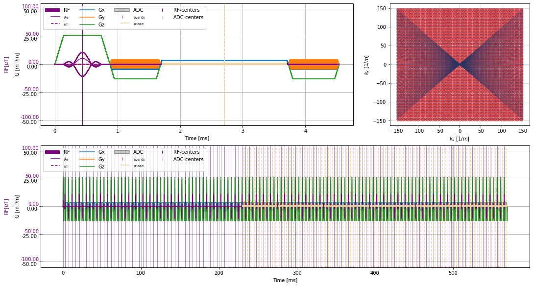
Illustrate sequence#
[8]:
plt.close("all")
f = plt.figure(constrained_layout=True, figsize=(15, 8))
axes = f.subplot_mosaic("AAB;CCC")

cmrseq.plotting.plot_sequence(seq_list[0], axes=axes["A"], format_axes=True, add_legend=False)
for s in seq_list[n_dummy:]:
    cmrseq.plotting.plot_sequence(s, axes=[f.axes[-1], axes["A"], axes["A"], axes["A"]], format_axes=False)
for s in seq_list[n_dummy:]:
    cmrseq.plotting.plot_kspace_2d(s, ax=axes["B"], k_axes=[0, 1])

full_seq = deepcopy(seq_list[0])
full_seq.extend(deepcopy(seq_list[1:]))
cmrseq.plotting.plot_sequence(full_seq, axes=axes["C"])
Extending Sequence: 100%|██████████| 125/125 [00:00<00:00, 336.01it/s]
Construct Phantom#
The geometrical relation of the phantom is defined in the custom function create_spherical_phantom. The RegularGridDataset class is used to compute the off-resonance maps as well as selecting a slice from the phantom to reduces the computational load during simulation (for isochromates permanently outside the excitation profile)
[9]:
phantom_ = local_functions.create_spherical_phantom(dimensions=(61, 61, 61), spacing=(0.004, 0.004, 0.004), big_radius=0.12)
phantom_["in_mesh"] = np.ones(phantom_.points.shape[0])


phantom = cmrsim.datasets.RegularGridDataset.from_unstructured_grid(phantom_, pixel_spacing=Quantity([1, 1, 1], "mm"),
                                                                    padding=Quantity([5, 5, 5], "cm"))
phantom.mesh["chi"] = np.where(phantom.mesh["in_mesh"], np.ones_like(phantom.mesh["in_mesh"]) * (-9.05),
                               np.ones_like(phantom.mesh["in_mesh"]) * 0.36) * 1e-6   # susceptibilty in ppm
phantom.compute_offresonance(b0=system_specs.b0, susceptibility_key="chi")
clear_output()


voxels = phantom.select_slice(slice_normal, spacing=Quantity([0.25, 0.25, 2], "mm"),
                              slice_position=slice_normal*slice_position_offset,
                              field_of_view=Quantity([*fov.m_as("m"), slice_thickness.m_as("m")*1.5], "m"),
                              readout_direction=readout_direction, in_mps=False)
voxels = voxels.threshold(0.1, "in_mesh")
/scratch/jweine/cmrsim/notebooks/bloch_simulation/../../cmrsim/utils/coordinates.py:96: UserWarning: Optimal rotation is not uniquely or poorly defined for the given sets of vectors.
  rot, _ = Rotation.align_vectors(original_basis, new_basis)
Illustrate the phantom within the coil-maps#
[10]:
# Create a clipped cylindrical mesh to 3D-render the coil-sensitvities
coil_maps = coil_module.coil_maps
coilmaps_magn = {f"mag_coil_{i}": np.abs(coil_maps[..., i]) for i in range(coil_maps.shape[-1])}
coilmaps_phase = {f"phi_coil_{i}": np.angle(coil_maps[..., i]) * 0 for i in range(coil_maps.shape[-1])}
coil_maps = dict(**coilmaps_magn, **coilmaps_phase)
coil_dataset = cmrsim.datasets.RegularGridDataset.from_numpy(data=coil_maps, extent=Quantity([60, 60, 90], "cm"))
cylinder = pyvista.Cylinder(center=(0., 0., 0.), direction=(0., 0., 1.), radius=0.15, height=0.4)
cylinder = coil_dataset.mesh.clip_surface(cylinder.extract_surface())
full_sphere = coil_dataset.mesh.probe(phantom_)
[11]:
import imageio

# Create the images
images = []
for coil_id in range(8):
    pyvista.close_all()
    pyvista.start_xvfb()
    plotter = pyvista.Plotter(off_screen=True, window_size=(300, 300))
    plotter.add_mesh(voxels, color="white")
    plotter.add_mesh(full_sphere, scalars=f"mag_coil_{coil_id}", cmap="plasma", opacity=0.9)
    plotter.add_mesh(cylinder, scalars=f"mag_coil_{coil_id}", cmap="plasma", show_scalar_bar=False, opacity=0.8)
    local_functions.add_custom_axes(plotter, scale=0.3)
    plotter.add_title(f"Coil #{coil_id}", font_size=8)
    images.append(plotter.screenshot(f"coil_rendering.png"))

ims = np.concatenate(np.concatenate(np.stack(images).reshape(2, 4, 300, 300, 3), axis=1), axis=1)
imageio.v3.imwrite("coil_rendering.png", ims)
b64 = base64.b64encode(open("coil_rendering.png",'rb').read()).decode('ascii')
display(HTML(f'<img src="data:image/gif;base64,{b64}" />'))

Instantiate Simulation Operators#
The dummy-shots of the sequence should not be run using the ParallelReceiveBlochOperator, because no sampling events are defined. Therefore, the sequnce definition is split at the first non-dummy shot. The first part is used to instantiate a GeneralBlochOperator while the second part is used to instantiate a ParallelReceiveBlochOperator which takes the coil-sensitivities created above as argument.
[12]:
# Split the dummyshots and create single Sequence instance
dummy_sequence = deepcopy(seq_list[0])
dummy_sequence.extend(seq_list[1:n_dummy+1])

# Grid the sequence definitions
time_dummy, rf_grid_dummy, grad_grid_dummy, _ = [np.stack(v) for v in cmrseq.utils.grid_sequence_list([dummy_sequence, ])]
time, rf_grid, grad_grid, adc_on_grid = [np.stack(v) for v in cmrseq.utils.grid_sequence_list(seq_list[n_dummy+1:])]

# Define off-resonsance submodule
offres = cmrsim.bloch.submodules.OffResonance(gamma=system_specs.gamma.m_as("MHz/T"), device="GPU:0")

# Construct BlochOperators and pass offresonance module:
module_dummyshots = cmrsim.bloch.GeneralBlochOperator(name="dummy_shots", gamma=system_specs.gamma_rad.m_as("rad/mT/ms"),
                                                      time_grid=time_dummy[0],
                                                      gradient_waveforms=grad_grid_dummy,
                                                      rf_waveforms=rf_grid_dummy,
                                                      device="GPU:0",
                                                      submodules=[offres, ]
                                                     )

module_acquisition = cmrsim.bloch.ParallelReceiveBlochOperator(name="acquisition", gamma=system_specs.gamma_rad.m_as("rad/mT/ms"),
                                                               coil_module=coil_module,
                                                               time_grid=time[0],
                                                               gradient_waveforms=grad_grid,
                                                               rf_waveforms=rf_grid,
                                                               adc_events=adc_on_grid,
                                                               device="GPU:0",
                                                               submodules=[offres, ]
                                                              )
Extending Sequence: 100%|██████████| 50/50 [00:00<00:00, 232.03it/s]
Prepare simulation input#
[13]:
n_particles = voxels.points.shape[0]
voxels["M0"] =np.ones(n_particles, dtype=np.float32)
voxels["T1"] =np.ones(n_particles, dtype=np.float32) * 1000
voxels["T2"] =np.ones(n_particles, dtype=np.float32) * 200

slice_dataset = cmrsim.datasets.RegularGridDataset(voxels)
properties = slice_dataset.get_phantom_def(filter_by="in_mesh", keys=["M0", "T1", "T2", "offres"],
                                           perturb_positions_std=Quantity(0.005, "mm").m_as("m"))
properties["initial_position"] = properties.pop("r_vectors")
properties["off_res"] = properties.pop("offres").reshape(-1, 1)
properties["magnetization"] = cmrsim.utils.particle_properties.norm_magnetization()(n_particles)

input_dataset = cmrsim.datasets.BlochDataset(properties, filter_inputs=True)
print([v["initial_position"].shape for v in input_dataset(batchsize=int(3e6)).take(1)])
[TensorShape([2667392, 3])]
Run simulation#
[14]:
# Instantiate simulator:
print(f"Total time-steps per TR: {time.shape[1]}")

for batch in tqdm(input_dataset(batchsize=int(3e6)).take(1)):
    print({k:v.shape for k, v in batch.items()})
    m_init = batch.pop("magnetization")
    initial_position = batch.pop("initial_position")
    m, r = module_dummyshots(initial_position=initial_position, magnetization=m_init, **batch)
    for tr_index in tqdm(range(time.shape[0]), desc="Iterating TRs", leave=False):
        m, r = module_acquisition(initial_position=r, magnetization=m, repetition_index=tr_index, **batch)
Total time-steps per TR: 505
{'M0': TensorShape([2667392]), 'T1': TensorShape([2667392]), 'T2': TensorShape([2667392]), 'initial_position': TensorShape([2667392, 3]), 'off_res': TensorShape([2667392, 1]), 'magnetization': TensorShape([2667392, 3])}
2023-01-13 12:27:13.468718: I tensorflow/compiler/xla/service/service.cc:173] XLA service 0x55b7b26249b0 initialized for platform CUDA (this does not guarantee that XLA will be used). Devices:
2023-01-13 12:27:13.468810: I tensorflow/compiler/xla/service/service.cc:181]   StreamExecutor device (0): NVIDIA TITAN RTX, Compute Capability 7.5
2023-01-13 12:27:13.480438: I tensorflow/compiler/mlir/tensorflow/utils/dump_mlir_util.cc:268] disabling MLIR crash reproducer, set env var `MLIR_CRASH_REPRODUCER_DIRECTORY` to enable.
2023-01-13 12:27:13.607806: I tensorflow/tsl/platform/default/subprocess.cc:304] Start cannot spawn child process: No such file or directory
2023-01-13 12:27:14.298168: I tensorflow/compiler/jit/xla_compilation_cache.cc:477] Compiled cluster using XLA!  This line is logged at most once for the lifetime of the process.
2023-01-13 12:29:30.467251: W tensorflow/compiler/tf2xla/kernels/assert_op.cc:38] Ignoring Assert operator linear_interpolation_lookup/Assert/Assert
Reconstruction#
First generate coil-map images by probing the 3D sensitivity maps (again using the functionality provided by the RegularGridDataset class).
[15]:
# Create coil-maps from the original input mesh
sl_mesh = coil_dataset.select_slice(slice_normal, spacing=Quantity([*res.m_as("m"), slice_thickness.m_as("m")], "m"),
                                    slice_position=slice_normal*slice_position_offset,
                                    field_of_view=Quantity([*fov.m_as("m"), slice_thickness.m_as("m")], "m"),
                                    readout_direction=readout_direction, in_mps=True)

coil_sensitivity_images = np.stack([sl_mesh[f"mag_coil_{i}"] + 1j * sl_mesh[f"phi_coil_{i}"] for i in range(8)], axis=-1).reshape(*matrix_size, 8, order="F")
/scratch/jweine/cmrsim/notebooks/bloch_simulation/../../cmrsim/utils/coordinates.py:96: UserWarning: Optimal rotation is not uniquely or poorly defined for the given sets of vectors.
  rot, _ = Rotation.align_vectors(original_basis, new_basis)
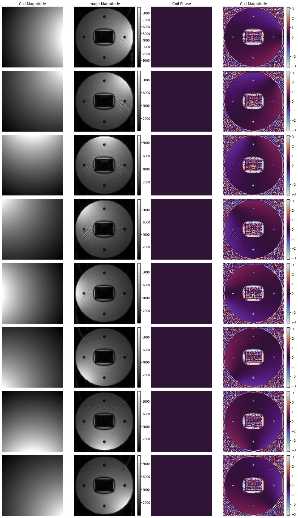
Now reconstruct each coil-channel separately and plot the result side-by-side with the reference sensitivity maps
[17]:
# Show images
fig, axes = plt.subplots(8, 4, figsize=(14, 24))

for i in range(8):
    time_signal = tf.stack([v[:, i] for v in module_acquisition.time_signal_acc], axis=0).numpy().reshape(*matrix_size[::-1], order="C")
    time_signal += tf.complex(*[tf.random.normal(shape=time_signal.shape, stddev=40) for i in range(2)])
    centered_projection = tf.signal.fft(time_signal).numpy()
    centered_k_space = tf.signal.fft(centered_projection).numpy()
    image = tf.signal.fftshift(tf.signal.ifft2d(tf.roll(tf.signal.ifftshift(centered_k_space, axes=(0, 1)), -1, axis=1)), axes=(0, 1)).numpy() * (0 + 1j)

    coil_mag = axes[i, 0].imshow(np.abs(coil_sensitivity_images[..., i]).T, cmap="gray")
    abs_plot = axes[i, 1].imshow(np.abs(np.squeeze(image)), cmap="gray")
    fig.colorbar(abs_plot, ax=axes[i, 1], fraction=0.045, pad=0.04)

    coil_phase = axes[i, 2].imshow(np.angle(coil_sensitivity_images[..., i]).T, cmap="twilight",  vmin=-np.pi, vmax=np.pi)
    phase_plot = axes[i, 3].imshow(np.angle(np.squeeze(image)), cmap="twilight", vmin=-np.pi, vmax=np.pi)
    fig.colorbar(phase_plot, ax=axes[i, 3], fraction=0.045, pad=0.04)
    [_.axis("off") for _ in axes[i]]

[_.set_title(t) for _, t in zip(axes[0], ["Coil Magnitude", "Image Magnitude", "Coil Phase", "Coil Magnitude"])]
fig.tight_layout()
[ ]: