Flow BSSFP#
Import modules and set TF-GPU configuration#
[1]:
import os
os.environ['TF_CPP_MIN_LOG_LEVEL'] = '2'

# Load TF and check for GPUs
import tensorflow as tf
gpus = tf.config.list_physical_devices('GPU')
for gpu in gpus:
    tf.config.experimental.set_memory_growth(gpu, True)
logical_gpus = tf.config.list_logical_devices('GPU')
print(len(gpus), "Physical GPUs,", len(logical_gpus), "Logical GPUs")

# 3rd Party dependencies
import cmrseq
from pint import Quantity
import pyvista
import numpy as np
import matplotlib.pyplot as plt
%matplotlib inline

# # Project library cmrsim
import sys
sys.path.append("../../")
import cmrsim
import cmrsim.utils.particle_properties as part_factory
1 Physical GPUs, 1 Logical GPUs
Section 1: Define & Run the Simulation#
Define Geometrical & Sequence parameters for simulation#
[2]:
# Define MR-system specifications
system_specs = cmrseq.SystemSpec(max_grad=Quantity(50, "mT/m"), max_slew=Quantity(200., "mT/m/ms"),
                                 grad_raster_time=Quantity(0.01, "ms"),
                                 rf_raster_time=Quantity(0.01, "ms"),
                                 adc_raster_time=Quantity(0.01,"ms"))

# Define Fourier-Encoding parameters
fov = Quantity([194, 122], "mm")
matrix_size = (97, 61)
res = fov / matrix_size
print("Resolution:", res)
n_dummy = 25
center_index = np.array(matrix_size) // 2 + np.mod(matrix_size, 2)
print(center_index)

# Define imaging slice parameters
slice_thickness = Quantity(6, "mm")
slice_position = Quantity([0., 0., 0.], "m")
adc_duration=Quantity(4., "ms")
readout_direction = np.array([0., 0., 1.]) # readout along scanner Z, (FH)
slice_normal = np.array([0., 1., 0.])
slice_position_offset = Quantity(0.5, "cm")

# Define RF-exication parameters (coupled with seeding slice atm)
flip_angle=Quantity(np.pi/4, "rad")
pulse_duration = Quantity(1., "ms")
RF_slice_normal = np.array([0., 1., 0.]) # Slice along scanner Y, (AP)
RF_slice_position = Quantity([0., 0., 0.], "m")
FA = np.pi/4

# Define Reseeding slice parameters
seeding_slice_position = Quantity([0.03, 0.005, -0.025], "m")
seeding_slice_normal = np.array([0.3, 0., 1.])
seeding_slice_thickness = Quantity(35, "mm")
seeding_pixel_spacing = np.array((0.5e-3, 0.5e-3, 0.5e-3)) # resolution of seeding mesh, mm
seeding_slice_bb = Quantity([6, 6, 4], "cm")
seeding_particle_density = 10 # per 1/mm*3

# Define initial filling
initial_fill_normal = np.array([0., 1., 0.])
initial_fill_position = Quantity([0., 0.005, 0.], "m")
initial_fill_thickness = Quantity(50, "mm")
initial_fill_bounding_box = Quantity([25, 25, 25], "cm")
lookup_mesh_spacing = np.array((0.5e-3, 0.5e-3, 0.5e-3)) # resolution of lookup mesh, mm
Resolution: [2.0 2.0] millimeter
[49 31]
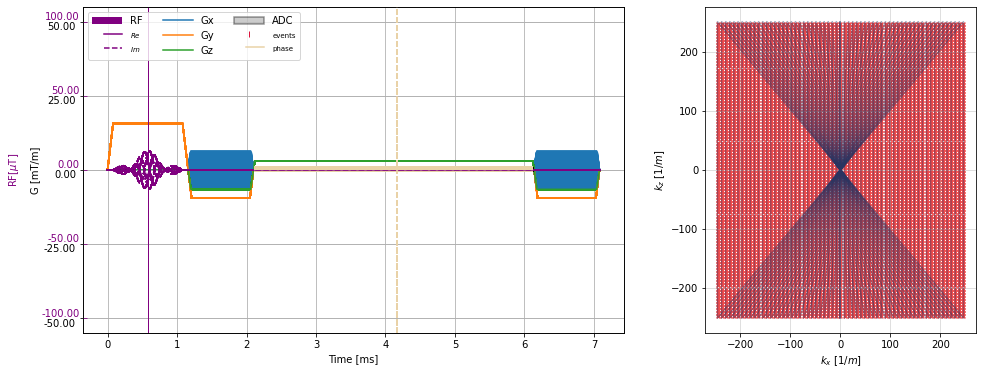
Set up Gradient, RF and ADC definitions#
[3]:
seq_list = cmrseq.seqdefs.sequences.balanced_ssfp(system_specs,
                                             matrix_size,
                                             inplane_resolution=res,
                                             slice_thickness=slice_thickness,
                                             adc_duration=adc_duration,
                                             flip_angle=flip_angle,
                                             pulse_duration=pulse_duration,
                                             slice_position_offset=slice_position_offset,
                                             dummy_shots=n_dummy)

rf_rotation_matrix = cmrseq.utils.get_rotation_matrix(RF_slice_normal, np.array([0., 0., 1.]))
ro_rotation_matrix = cmrseq.utils.get_rotation_matrix(slice_normal, readout_direction)

for rep_idx, seq in enumerate(seq_list):
    # Rotate subsequences according to slice definition
    rf_blocks = cmrseq.utils.get_partial_sequence(seq, seq.blocks[0:4], copy=False)
    rf_blocks.rotate_gradients(rf_rotation_matrix)
    ro_blocks = cmrseq.utils.get_partial_sequence(seq, seq.blocks[4:], copy=False)
    ro_blocks.rotate_gradients(ro_rotation_matrix)

_, k_adc, t_adc = seq_list[n_dummy + center_index[1]].calculate_kspace()

plt.close("all")
f, (a1, a2) = plt.subplots(1, 2, figsize=(16, 6), gridspec_kw={"width_ratios":(2, 1)})

cmrseq.plotting.plot_sequence(seq_list[0], axes=a1, format_axes=True)
for s in seq_list[n_dummy:]:
    cmrseq.plotting.plot_sequence(s, axes=[f.axes[-1], a1, a1, a1], format_axes=False)
for s in seq_list[n_dummy:]:
    cmrseq.plotting.plot_kspace_2d(s, ax=a2, k_axes=[0, 2])
/scratch/jweine/conda/envs/tf29_pyvista/lib/python3.9/site-packages/pint/quantity.py:1313: RuntimeWarning: invalid value encountered in double_scalars
  magnitude = magnitude_op(new_self._magnitude, other._magnitude)
[4]:
from cmrsim.simulation_templates.flow import FlowSimulation


# Define off-resonsance and T2* modules
offres = cmrsim.bloch.submodules.OffResonance(gamma=system_specs.gamma.m_as("MHz/T"), device="GPU:0")
T2s = cmrsim.bloch.submodules.T2starDistributionModel()

submodules = [T2s,offres]


time_cat, rf_grid_cat, grad_grid_cat, _ = [np.stack(v) for v in cmrseq.utils.grid_sequence_list([seq_list[0]], force_uniform_grid=False)]
time_dummy, rf_grid_dummy, grad_grid_dummy, _ = [np.stack(v) for v in cmrseq.utils.grid_sequence_list(seq_list[1:(n_dummy+1)], force_uniform_grid=False)]
time, rf_grid, grad_grid, adc_on_grid = [np.stack(v) for v in cmrseq.utils.grid_sequence_list(seq_list[(n_dummy+1):], force_uniform_grid=False)]

print(time.shape, rf_grid.shape, grad_grid.shape, adc_on_grid.shape)

bloch_catalyst = cmrsim.bloch.GeneralBlochOperator(name="rf", gamma=system_specs.gamma_rad.m_as("rad/mT/ms"),
                                                 time_grid=time_cat[0], gradient_waveforms=grad_grid_cat,
                                                 rf_waveforms=rf_grid_cat, device="GPU:0",
                                                 submodules=submodules)

bloch_dummy = cmrsim.bloch.GeneralBlochOperator(name="rf", gamma=system_specs.gamma_rad.m_as("rad/mT/ms"),
                                                 time_grid=time_dummy[0], gradient_waveforms=grad_grid_dummy,
                                                 rf_waveforms=rf_grid_dummy, device="GPU:0",
                                                 submodules=submodules)

bloch_readout = cmrsim.bloch.GeneralBlochOperator(name="rf", gamma=system_specs.gamma_rad.m_as("rad/mT/ms"),
                                                 time_grid=time[0], gradient_waveforms=grad_grid,
                                                 rf_waveforms=rf_grid, adc_events=adc_on_grid, device="GPU:0",
                                                 submodules=submodules)
(61, 805) (61, 805) (61, 805, 3) (61, 805, 2)
Load Mesh & Instantiate Dataset object#
[5]:
# Load Aorta Example.
mesh = pyvista.read("../example_resources/pv_computed_averaged_P14.vtk")

# The velocity [m/s] is stored in the mesh as U1. In cmrsim all definitions are done in [ms] therefore
# We add the velocity field as scaled data to the mesh
mesh["velocity"] = Quantity(mesh["U1"], "m/s").m_as("m/ms") * 0.4

# To match the usual geometry (Head <-> Foot along z-axis) flip the axes of the mesh
mesh.points = mesh.points[:,[2,1,0]]
mesh.points[:, 1:] *= -1
mesh["velocity"] = mesh["velocity"][:,[2,1,0]]
mesh["velocity"][:, 1:] *= -1
global_mesh_offset = [0.02, 0.01, -0.02]
mesh.translate(global_mesh_offset, inplace=True)

# Rotate mesh and flow by 60 degrees
mesh.rotate_z(60, (0., 0., 0.), inplace=True)
vx = np.cos(60*np.pi/180)*mesh["velocity"][:,0] - np.sin(60*np.pi/180)*mesh["velocity"][:,1]
mesh["velocity"][:,1] = np.sin(60*np.pi/180)*mesh["velocity"][:,0] + np.cos(60*np.pi/180)*mesh["velocity"][:,1]
mesh["velocity"][:,0] = vx

mesh = mesh.cell_data_to_point_data()

# clip to restricted length to reduce mesh-size
mesh.clip(normal='z', origin=[0., 0., 0.09], inplace=True)
mesh.clip(normal='-z', origin=[0., 0., -0.09], inplace=True)

# setup initial fill dictionary

initial_fill_dict = {'slice_normal':initial_fill_normal,
                     'slice_position':initial_fill_position.m_as('m'),
                     'slice_thickness':initial_fill_thickness.m_as('m'),
                     'slice_bounding_box':initial_fill_bounding_box.m_as('m')}

# Add artificial channel for off_resonance
TR = seq_list[-1].duration
#banding_dist = Quantity(4.5, "cm")
#mesh["off_res"] = mesh.points[:, 2] / banding_dist.m_as("m") * 2 / TR.m_as("ms") / system_specs.gamma.m_as("MHz/T")
mesh["off_res"] = (mesh.points[:, 0]<0) /2/ TR.m_as("ms") / system_specs.gamma.m_as("MHz/T")

# Setup flow dataset with seeding mesh information
# Here T1, T2 and T2' are set
particle_creation_fncs = {"magnetization": part_factory.norm_magnetization(),
                          "T1": part_factory.uniform(default_value=1000.),
                          "T2": part_factory.uniform(default_value=200.),
                          "omega_t2s": part_factory.t2star_lorentzian(T2p = 40,prctile_cutoff=0.002),
                          "M0": part_factory.uniform(default_value=1/seeding_particle_density)}

dataset = cmrsim.datasets.RefillingFlowDataset(mesh,
                                               particle_creation_callables=particle_creation_fncs,
                                               slice_position=seeding_slice_position.m_as("m"),
                                               slice_normal=seeding_slice_normal,
                                               slice_thickness=seeding_slice_thickness.m_as("m"),
                                               slice_bounding_box=seeding_slice_bb.m_as("m"),
                                               seeding_vol_spacing=seeding_pixel_spacing,
                                               lookup_map_spacing=lookup_mesh_spacing,
                                               field_list=[("velocity", 3), ("off_res", 1)])
mesh
Updated Mesh
Updated Slice Position
[5]:
| Header | Data Arrays | ||||||||||||||||||||||||||||||||||||||||||||
|---|---|---|---|---|---|---|---|---|---|---|---|---|---|---|---|---|---|---|---|---|---|---|---|---|---|---|---|---|---|---|---|---|---|---|---|---|---|---|---|---|---|---|---|---|---|
|
|
Optional: Check Slice configuration#
[ ]:
pyvista.close_all()
pyvista.set_jupyter_backend('panel')
pyvista.start_xvfb()
plotter = pyvista.Plotter(notebook=True, window_size=(500, 750))

# Plot axes at origin
origin_arrows = [pyvista.Arrow(start=(0., 0., 0.), direction=direction, tip_length=0.1, tip_radius=0.025,
                               tip_resolution=10, shaft_radius=0.005, shaft_resolution=10, scale=0.1)
                 for direction in [(1., 0., 0.), (0., 1., 0.), (0., 0., 1.)]]
plotter.add_mesh(origin_arrows[0], color="blue", label="x")
plotter.add_mesh(origin_arrows[1], color="green", label="y")
plotter.add_mesh(origin_arrows[2], color="red", label="z")

# Plot input mesh
#plotter.add_mesh(mesh, scalars="velocity", opacity=1)
plotter.add_mesh(mesh, scalars="off_res", opacity=1)

# Plot slice selective RF
_scale = 0.1
rf_mesh = pyvista.Box(bounds=(-_scale, _scale, -_scale, _scale, -slice_thickness.m_as("m")/2, slice_thickness.m_as("m")/2))
rf_mesh.points = cmrseq.utils.mps_to_xyz(rf_mesh.points[np.newaxis], slice_normal=RF_slice_normal, readout_direction=np.array([1., 0., 0.]))[0]
rf_mesh.translate(RF_slice_normal * slice_position_offset.m_as("m"), inplace=True)
plotter.add_mesh(rf_mesh, opacity=0.1, show_edges=True, color="red")

# Plot projection plane of the cartesian image slice with M-S directions
image_slice_mesh = pyvista.Box(bounds=(-fov[0].m_as("m")/2, fov[0].m_as("m")/2, -fov[1].m_as("m")/2, fov[1].m_as("m")/2, 0, 0))
image_slice_mesh.points = cmrseq.utils.mps_to_xyz(image_slice_mesh.points[np.newaxis], slice_normal=slice_normal, readout_direction=readout_direction)[0]
readout_glyph = pyvista.Arrow(start=slice_position.m_as("m"), direction=readout_direction, tip_length=0.1, tip_radius=0.025,
                               tip_resolution=10, shaft_radius=0.01, shaft_resolution=10, scale=0.05)
slice_selection_glyph = pyvista.Arrow(start=slice_position.m_as("m"), direction=slice_normal, tip_length=0.1, tip_radius=0.025,
                               tip_resolution=10, shaft_radius=0.01, shaft_resolution=10, scale=0.05)

plotter.add_mesh(image_slice_mesh, opacity=1, show_edges=True)
plotter.add_mesh(readout_glyph, color="black")
plotter.add_mesh(slice_selection_glyph, color="black")

# Add Initial fill volume

_scale = 0.1
inf_mesh = pyvista.Box(bounds=(-_scale, _scale, -_scale, _scale, -initial_fill_thickness.m_as("m")/2, initial_fill_thickness.m_as("m")/2))
inf_mesh.points = cmrseq.utils.mps_to_xyz(inf_mesh.points[np.newaxis], slice_normal=initial_fill_normal, readout_direction=np.array([0., 0., 1.]))[0]
inf_mesh.translate(initial_fill_position.m_as("m"), inplace=True)
plotter.add_mesh(inf_mesh, opacity=0.1, show_edges=True, color="green")

# Plot the slice in which the re-seeding is performed
plotter.add_mesh(dataset.gridded_seeding_volume, color="orange", opacity=0.7)

# Plot reseeded particles
#test_particles, test_properties, _ = dataset(particle_density=0.1)

# r, v = simulator.trajectory_module.call_with_velocity(tf.constant(test_particles), dt=0.1, n_steps=n_steps_total)
# rnew, _, in_tol = dataset(particle_density=0.1, residual_particle_pos=r[:, -1], particle_properties=test_properties,
#                           reseed_threshold=0., distance_tolerance=0.05)
# print(in_tol[0].shape)
# print(dataset.n_new, rnew.shape[0], np.delete(rnew, in_tol, axis=0).shape)

# plotter.add_mesh(pyvista.PolyData(r[-1]), scalars=np.linalg.norm(v[-1], axis=-1))
# plotter.add_mesh(pyvista.PolyData(np.delete(rnew, in_tol, axis=0)), color="gray")
# plotter.add_mesh(pyvista.PolyData(r[0]), scalars=np.linalg.norm(v[0], axis=-1))
plotter.show()
Run Simulation#
[6]:
# Instantiate simulator:
simulator = FlowSimulation(flow_dataset=dataset, prep_modules=[bloch_catalyst,bloch_dummy],readout_module=bloch_readout)
n_steps_total = grad_grid.shape[1]

print(f"Total time-steps per TR: {n_steps_total}")
r,m = simulator(particle_density=seeding_particle_density,
                dropping_distance=0.15, averages=1,
                reseed_threshold=0.3, use_inital_filling=True,
                initial_filling_dict=initial_fill_dict,
                return_final_magnetization=True)
Total time-steps per TR: 805
Section 2: Visualize Results#
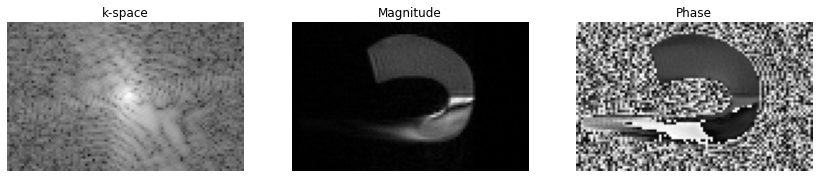
First obtain the accumulated time-domain signal from the encoding module. This signal is discretized on the simulation raster. The encoding module yields the centered spatial projection corresponding to the time-domain signals fourier transform.
To obtain the projection with “removed oversampling” the projections are linearly interpolated to the positions corresponding to the instantaneous encoding times t_adc as defined above. By calling the encoding modules get_kspace() these cropped projections are again fourier transformed, yielding the 2D cartesian k-space.
[7]:
time_signal = tf.stack(bloch_readout.time_signal_acc, axis=0).numpy().reshape(matrix_size[::-1])

# Add noise based on max (DC) time signal at SNR of >100. This does not affect the magnitude image,
#     but the phase image will not have structures in regions of zero signal
n = (np.random.normal(0,1,time_signal.shape))*np.max(np.abs(time_signal))/1000
n = n*np.exp(1j*np.random.normal(0,1,time_signal.shape))
time_signal = time_signal +n

centered_projection = tf.signal.fft(time_signal).numpy()
centered_k_space = tf.signal.fft(centered_projection).numpy()
image = tf.signal.fftshift(tf.signal.ifft2d(tf.roll(tf.signal.ifftshift(centered_k_space, axes=(0, 1)),  -1, axis=1)), axes=(0,1)).numpy()
time_per_seg = t_adc - t_adc[center_index[0]]
freq_per_seg = np.fft.fftfreq(n=time_per_seg.shape[0], d=time_per_seg[1]-time_per_seg[0])

print(time_signal.shape, centered_projection.shape, time_per_seg.shape, freq_per_seg.shape, image.shape)
(61, 97) (61, 97) (97,) (97,) (61, 97)
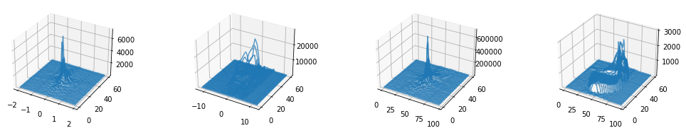
Plot 1 - 3D visualization of echo-signal in temporal domain processed into k-space lines#
[8]:
# Plot all PE-lines in 3D
plt.close("all")
from mpl_toolkits.mplot3d.axes3d import Axes3D
fig, axes = plt.subplots(1, 4, subplot_kw={'projection': '3d'}, figsize=(15, 2.5))
for ky in range(time_signal.shape[0]):
axes[0].plot(time_per_seg, np.ones_like(time_signal[ky].real) * ky, np.abs(time_signal[ky]), color="C0", linestyle="-", alpha=0.7)
axes[1].plot(freq_per_seg, np.ones_like(centered_projection[ky].real) * ky, np.abs(centered_projection[ky]), color="C0", linestyle="-", alpha=0.7)
axes[2].plot(np.arange(freq_per_seg.shape[0]), np.ones_like(centered_k_space[ky].real) * ky, np.abs(centered_k_space[ky]), color="C0", linestyle="-", alpha=0.7)
axes[3].plot(np.arange(freq_per_seg.shape[0]), np.ones_like(image[ky].real) * ky, np.abs(image[ky]), color="C0", linestyle="-", alpha=0.7)
fig.tight_layout()
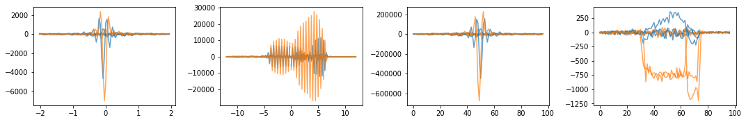
# Plot 2D Lines
fig, axes = plt.subplots(1, 4, figsize=(15, 2.5))
for ky in range(0, 31, 10):
axes[0].plot(time_per_seg, np.real(time_signal[ky]), color="C0", linestyle="-", alpha=0.7)
axes[0].plot(time_per_seg, np.imag(time_signal[ky]), color="C1", linestyle="-", alpha=0.7)
axes[1].plot(freq_per_seg, np.real(centered_projection[ky]), color="C0", linestyle="-", alpha=0.7)
axes[1].plot(freq_per_seg, np.imag(centered_projection[ky]), color="C1", linestyle="-", alpha=0.7)
axes[2].plot(np.arange(freq_per_seg.shape[0]), np.real(centered_k_space[ky]), color="C0", linestyle="-", alpha=0.7)
axes[2].plot(np.arange(freq_per_seg.shape[0]), np.imag(centered_k_space[ky]), color="C1", linestyle="-", alpha=0.7)
axes[3].plot(np.arange(freq_per_seg.shape[0]), np.real(image[ky]), color="C0", linestyle="-", alpha=0.7)
axes[3].plot(np.arange(freq_per_seg.shape[0]), np.imag(image[ky]), color="C1", linestyle="-", alpha=0.7)
fig.tight_layout()
# Show images
fig, axes = plt.subplots(1, 3, figsize=(12, 2.5))
axes[0].imshow(np.log(np.abs(np.squeeze(centered_k_space))), cmap="gray")
axes[1].imshow(np.abs(np.squeeze(image)), cmap="gray")
axes[2].imshow(np.angle(np.squeeze(image)), cmap="gray")
[_.axis("off") for _ in axes]
[_.set_title(t) for _, t in zip(axes, ["k-space", "Magnitude", "Phase"])]
fig.tight_layout()
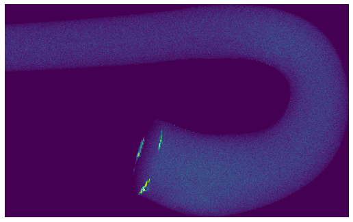
Visualize final particle density#
This is a good way to ensure that there are no reseeding or particle trajectory errors, such as density voids or pileups
[9]:
fig, axes = plt.subplots(1, 1, figsize=(9, 5))

plot_axes = [0,2] # Change these to change the axes of the projection

A,xe,ye,_ = plt.hist2d(r[:,plot_axes[0]],r[:,plot_axes[1]],600)
fig.clear()
asp = (np.max(xe) - np.min(xe)) / (np.max(ye) - np.min(ye)) * 9
fig.set_size_inches(9,asp)
plt.imshow(A,aspect='auto',vmin=0,vmax=50)
plt.axis('off')
plt.show()