Spin Echo with Single Shot EPI#
In this notebook the sequence is composed with cmrseq and the input is a shepp-logan phantom, constructed with the phantominator package link
Imports#
[1]:
import sys
sys.path.append("../..")
from copy import deepcopy

# Load TF and check for GPUs
import tensorflow as tf
physical_devices = tf.config.list_physical_devices('GPU')
if physical_devices:
    print("Available GPUS: \n\t", "\n\t".join([str(_) for _ in physical_devices]))
    tf.config.experimental.set_visible_devices(physical_devices[1], 'GPU')
    tf.config.experimental.set_memory_growth(physical_devices[1], True)

# 3rd Party dependencies
import matplotlib.pyplot as plt
%matplotlib inline
from tqdm.notebook import tqdm
from pint import Quantity
import pyvista
import numpy as np
import cmrseq

# Project library cmrsim
import cmrsim
from cmrsim.utils import particle_properties as part_factory
Available GPUS:
         PhysicalDevice(name='/physical_device:GPU:0', device_type='GPU')
        PhysicalDevice(name='/physical_device:GPU:1', device_type='GPU')
        PhysicalDevice(name='/physical_device:GPU:2', device_type='GPU')
2022-08-17 15:48:11.964954: I tensorflow/core/platform/cpu_feature_guard.cc:193] This TensorFlow binary is optimized with oneAPI Deep Neural Network Library (oneDNN) to use the following CPU instructions in performance-critical operations:  AVX2 AVX512F FMA
To enable them in other operations, rebuild TensorFlow with the appropriate compiler flags.
2022-08-17 15:48:12.528464: I tensorflow/core/common_runtime/gpu/gpu_device.cc:1532] Created device /job:localhost/replica:0/task:0/device:GPU:0 with 22684 MB memory:  -> device: 1, name: NVIDIA TITAN RTX, pci bus id: 0000:3d:00.0, compute capability: 7.5
Construct Sequence#
[2]:
# Define MR-system specifications
system_specs = cmrseq.SystemSpec(max_grad=Quantity(40, "mT/m"), max_slew=Quantity(200., "mT/m/ms"),
                                 grad_raster_time=Quantity(0.01, "ms"),
                                 rf_raster_time=Quantity(0.01, "ms"),
                                 adc_raster_time=Quantity(0.01, "ms"))

fov = Quantity([200, 200], "mm")
matrix_size = (25, 25)
res = fov / matrix_size
adc_duration = Quantity(2., "ms")
pulse_duration = Quantity(1.5, "ms")
slice_thickness = Quantity(2, "cm")
flip_angle = Quantity(12, "degree").to("rad")

print("Resolution:", res)
Resolution: [8.0 8.0] millimeter
[3]:
partial_fourier_lines = 0
single_shot_epi = cmrseq.parametric_definitions.readout.epi_cartesian(system_specs, field_of_view=fov, matrix_size=matrix_size,
                                                                      blip_direction="up", partial_fourier_lines=partial_fourier_lines,
                                                                      adc_duration=Quantity(0.6, "ms"))

# Calculate duration to k-space center for echotime
k_grad, k_adc, t_adc = single_shot_epi.calculate_kspace()
n_klines_before_echo = matrix_size[1] // 2 - partial_fourier_lines
center_idx = n_klines_before_echo * matrix_size[0] + matrix_size[0] // 2
k_center, t_center = k_adc[:, center_idx], t_adc[center_idx]
t_center =  Quantity(t_center, "ms")
t_past = system_specs.time_to_raster(single_shot_epi.duration - t_center)
t_diff = system_specs.time_to_raster(t_past - t_center)

print(center_idx, k_center, t_center, t_past, single_shot_epi.duration)

spin_echo = cmrseq.parametric_definitions.excitation.slice_selective_se_pulses(system_specs, echo_time=Quantity(120, "ms"),
                                                                               slice_thickness=slice_thickness,
                                                                               pulse_duration=pulse_duration,
                                                                               slice_orientation=np.array([0., 0., 1.]),
                                                                               time_bandwidth_product=6)
center_first_pulse = spin_echo.get_block("ss_sinc_rf_0").rf_events[0]
min_echo_time = system_specs.time_to_raster(t_center * 2)
spin_echo = cmrseq.parametric_definitions.excitation.slice_selective_se_pulses(system_specs, echo_time=min_echo_time,
                                                                               slice_thickness=slice_thickness,
                                                                               pulse_duration=pulse_duration,
                                                                               slice_orientation=np.array([0., 0., 1.]),
                                                                               time_bandwidth_product=6)

se_ss_epi = deepcopy(spin_echo)
se_ss_epi.append(single_shot_epi)
312 [ 1.11022302e-15 -1.17437054e-01 0.00000000e+00] 8.72 millisecond 8.5 millisecond 17.22 millisecond
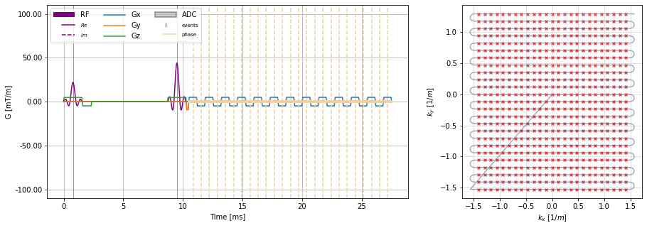
[8]:
# Plot Sequence
plt.close("all")
f, axes = plt.subplots(1, 2, figsize=(15, 5), gridspec_kw={"width_ratios":(2, 1)})
cmrseq.plotting.plot_sequence(se_ss_epi, axes=[axes[0],] * 4)
cmrseq.plotting.plot_kspace_2d(single_shot_epi, ax=axes[1])
[8]:
<AxesSubplot:xlabel='$k_x$ $[1/m]$', ylabel='$k_y$ $[1/m]$'>
Set up Phantom#
[9]:
import phantominator
x, y, z = 750, 750, 15
m0, t1, t2 = phantominator.shepp_logan(N=(x, y, z), MR=True, B0=1)

image_box = np.array((0.2, 0.2, 0.15))
dims = np.array([x, y, z])
resolution = image_box / dims
origin = - image_box / 2
uniform_grid = pyvista.UniformGrid(dims=dims, spacing=resolution, origin=origin)
uniform_grid["M0"] = m0.flatten(order="F")
uniform_grid["T1"] = t1.flatten(order="F") * 1000
uniform_grid["T2"] = t2.flatten(order="F") * 1000

uniform_grid
[9]:
| Header | Data Arrays | ||||||||||||||||||||||||||||||||||||||||||
|---|---|---|---|---|---|---|---|---|---|---|---|---|---|---|---|---|---|---|---|---|---|---|---|---|---|---|---|---|---|---|---|---|---|---|---|---|---|---|---|---|---|---|---|
|
|
[10]:
properties = {"M0":  uniform_grid["M0"].astype(np.float32),
              "T1":  uniform_grid["T1"].astype(np.float32),
              "T2":  uniform_grid["T2"].astype(np.float32),
              "magnetization": part_factory.norm_magnetization()(x*y*z),
              "initial_position": uniform_grid.points.astype(np.float32)
              }
input_dataset = cmrsim.datasets.BlochDataset(properties, filter_inputs=True)
surface_mesh = uniform_grid.threshold(0.1, scalars="M0")
Grid sequence and configure Bloch Module#
[12]:
t_comb, rf_comb, grad_comb, adc_on_comb = [np.stack(v) for v in cmrseq.utils.grid_sequence_list([se_ss_epi, ])]

print([v.shape for v in (t_comb, rf_comb, grad_comb, adc_on_comb)])

module_comb = cmrsim.bloch.GeneralBlochOperator(name="testmodule", gamma=system_specs.gamma_rad.m_as("rad/mT/ms"),
                                                time_grid=t_comb[0],
                                                gradient_waveforms=grad_comb,
                                                rf_waveforms=rf_comb,
                                                adc_events=adc_on_comb,
                                                device="GPU:0")
[(1, 3251), (1, 3251), (1, 3251, 3), (1, 3251, 2)]
Run Simulation#
[13]:
for batch in tqdm(input_dataset(batchsize=int(1e6))):
    _ = module_comb(repetition_index=0, **batch)
2022-08-17 15:51:58.681933: I tensorflow/compiler/xla/service/service.cc:170] XLA service 0x7f39e4b42f60 initialized for platform CUDA (this does not guarantee that XLA will be used). Devices:
2022-08-17 15:51:58.681977: I tensorflow/compiler/xla/service/service.cc:178]   StreamExecutor device (0): NVIDIA TITAN RTX, Compute Capability 7.5
2022-08-17 15:51:58.688669: I tensorflow/compiler/mlir/tensorflow/utils/dump_mlir_util.cc:263] disabling MLIR crash reproducer, set env var `MLIR_CRASH_REPRODUCER_DIRECTORY` to enable.
2022-08-17 15:51:59.491631: I tensorflow/core/platform/default/subprocess.cc:304] Start cannot spawn child process: No such file or directory
2022-08-17 15:52:00.035390: I tensorflow/compiler/jit/xla_compilation_cache.cc:478] Compiled cluster using XLA!  This line is logged at most once for the lifetime of the process.
Reconstruct Image#
[14]:
# Flip uneven k-space lines as they are acquired in "reversed" time
time_signal = tf.stack(module_comb.time_signal_acc, axis=0).numpy().reshape(matrix_size[::-1])
time_signal[1::2, :] = time_signal[1::2, ::-1]

centered_projection = tf.signal.fft(time_signal).numpy()
centered_k_space = tf.signal.fft(centered_projection).numpy()
image = tf.signal.fftshift(tf.signal.ifft2d(tf.roll(tf.signal.ifftshift(centered_k_space, axes=(0, 1)), (-1, -1), axis=(0, 1))), axes=(0, 1)).numpy() * (-1)
time_per_seg = t_adc[0:matrix_size[0]] - t_center.m_as("ms")
freq_per_seg = np.fft.fftfreq(n=time_per_seg.shape[0], d=time_per_seg[1]-time_per_seg[0])
print(time_signal.shape, centered_projection.shape, time_per_seg.shape, freq_per_seg.shape, image.shape)
(25, 25) (25, 25) (25,) (25,) (25, 25)
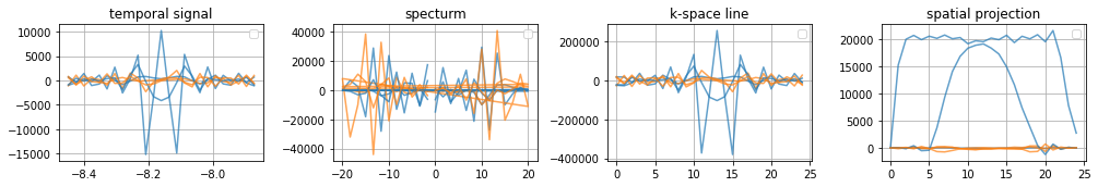
Plot 2D representation of specific single line acquisitions#
If the configured adc only acquires the exact k-space locations the acquired time signal equals the k-space line
[15]:
# Plot 2D Lines
fig, axes = plt.subplots(1, 4, figsize=(14, 2.5))
[a.grid(True) for a in axes]
[a.set_title(t) for a, t in zip(axes, ["temporal signal", "specturm", "k-space line", "spatial projection"])]
[a.legend(["real", "Imaginary"]) for a in axes]
for ky in range(0, time_signal.shape[0], 10):
    axes[0].plot(time_per_seg, np.real(time_signal[ky]), color="C0", linestyle="-", alpha=0.7)
    axes[0].plot(time_per_seg, np.imag(time_signal[ky]), color="C1", linestyle="-", alpha=0.7)
    axes[1].plot(freq_per_seg, np.real(centered_projection[ky]), color="C0", linestyle="-", alpha=0.7)
    axes[1].plot(freq_per_seg, np.imag(centered_projection[ky]), color="C1", linestyle="-", alpha=0.7)
    axes[2].plot(np.arange(freq_per_seg.shape[0]), np.real(centered_k_space[ky]), color="C0", linestyle="-", alpha=0.7)
    axes[2].plot(np.arange(freq_per_seg.shape[0]), np.imag(centered_k_space[ky]), color="C1", linestyle="-", alpha=0.7)
    axes[3].plot(np.arange(freq_per_seg.shape[0]), np.real(image[ky]), color="C0", linestyle="-", alpha=0.7)
    axes[3].plot(np.arange(freq_per_seg.shape[0]), np.imag(image[ky]), color="C1", linestyle="-", alpha=0.7)
fig.tight_layout()
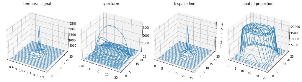
Plot 3D representation of simulation results#
If the configured adc only acquires the exact k-space locations the acquired time signal equals the k-space line
[16]:
# Plot all PE-lines in 3D
plt.close("all")
from mpl_toolkits.mplot3d.axes3d import Axes3D
fig, axes = plt.subplots(1, 4, subplot_kw={'projection': '3d'}, figsize=(14, 4))
[a.set_title(t) for a, t in zip(axes, ["temporal signal", "specturm", "k-space line", "spatial projection"])]

for ky in range(time_signal.shape[0]):
    axes[0].plot(time_per_seg, np.ones_like(time_signal[ky].real) * ky, np.abs(time_signal[ky]), color="C0", linestyle="-", alpha=0.7)
    axes[1].plot(freq_per_seg, np.ones_like(centered_projection[ky].real) * ky, np.abs(centered_projection[ky]), color="C0", linestyle="-", alpha=0.7)
    axes[2].plot(np.arange(freq_per_seg.shape[0]), np.ones_like(centered_k_space[ky].real) * ky, np.abs(centered_k_space[ky]), color="C0", linestyle="-", alpha=0.7)
    axes[3].plot(np.arange(freq_per_seg.shape[0]), np.ones_like(image[ky].real) * ky, np.abs(image[ky]), color="C0", linestyle="-", alpha=0.7)
fig.tight_layout()
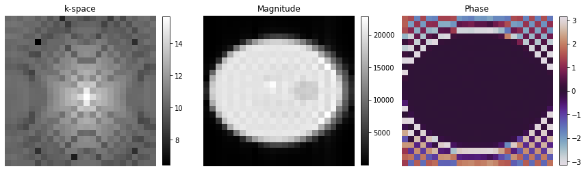
Plot Image#
[17]:
# Show images
fig, axes = plt.subplots(1, 3, figsize=(12, 5))

kspace_plot = axes[0].imshow(np.log(np.abs(np.squeeze(centered_k_space))), cmap="gray")
fig.colorbar(kspace_plot, ax=axes[0], fraction=0.045, pad=0.04)

abs_plot = axes[1].imshow(np.abs(np.squeeze(image)), cmap="gray")
fig.colorbar(abs_plot, ax=axes[1], fraction=0.045, pad=0.04)
phase_plot = axes[2].imshow(np.angle(np.squeeze(image)), cmap="twilight", vmin=-np.pi, vmax=np.pi)
fig.colorbar(phase_plot, ax=axes[2], fraction=0.045, pad=0.04)
[_.axis("off") for _ in axes]
[_.set_title(t) for _, t in zip(axes, ["k-space", "Magnitude", "Phase"])]
fig.tight_layout()