Static Phantom with off-resonance#
In this notebook, a simulation of a balanced steady state free precession with a spherical static phantom with air inclusions is performed. To do so the following steps are performed:
Define the Analytic Simulator
Define a 3D spherical phantom
Run simulation
Reconstruct images
Import modules and set TF-GPU configuration#
[1]:
from copy import deepcopy
import base64
from IPython.display import display, HTML, clear_output

# Load TF and check for GPUs
import tensorflow as tf
physical_devices = tf.config.list_physical_devices('GPU')
if physical_devices:
    print("Available GPUS: \n\t", "\n\t".join([str(_) for _ in physical_devices]))
    tf.config.experimental.set_visible_devices(physical_devices[0], 'GPU')
    tf.config.experimental.set_memory_growth(physical_devices[0], True)

# 3rd Party dependencies
import cmrseq
from pint import Quantity
import pyvista
import numpy as np
from tqdm.notebook import tqdm
import matplotlib.pyplot as plt
%matplotlib inline

# Project library cmrsim
import sys
sys.path.insert(0, "../../")
import cmrsim
import cmrsim.utils.particle_properties as part_factory
Available GPUS:
         PhysicalDevice(name='/physical_device:GPU:0', device_type='GPU')
2022-12-13 10:56:48.793905: I tensorflow/core/platform/cpu_feature_guard.cc:193] This TensorFlow binary is optimized with oneAPI Deep Neural Network Library (oneDNN) to use the following CPU instructions in performance-critical operations:  AVX2 AVX512F FMA
To enable them in other operations, rebuild TensorFlow with the appropriate compiler flags.
2022-12-13 10:56:49.438207: I tensorflow/core/common_runtime/gpu/gpu_device.cc:1532] Created device /job:localhost/replica:0/task:0/device:GPU:0 with 21480 MB memory:  -> device: 0, name: NVIDIA TITAN RTX, pci bus id: 0000:b2:00.0, compute capability: 7.5
1. Define Analytical Simulator#
[2]:
from typing import Tuple

class BSSFPSimulator(cmrsim.analytic.simulation.AnalyticSimulation):
    def build(self, fov: Tuple[float, float], matrix_size: Tuple[int, int], flip_angle: float, TE: float, TR: float,
              slice_thickness: Quantity = Quantity(10, "mm"), adc_duration: Quantity = Quantity(2, "ms"),
              pulse_duration: Quantity = Quantity(0.5, "ms")):
        n_kx, n_ky = matrix_size

        # Encoding definition
        inplane_resolution = Quantity(fov, "m") / matrix_size
        sequence_list = cmrseq.seqdefs.sequences.balanced_ssfp(cmrseq.SystemSpec(), matrix_size, inplane_resolution,
                                                               slice_thickness=slice_thickness, adc_duration=adc_duration,
                                                               flip_angle=Quantity(flip_angle, "degree"),
                                                               pulse_duration=pulse_duration)
        encoding_module = cmrsim.analytic.encoding.GenericEncoding(name="bssfp_readout", sequence=sequence_list[1:], absolute_noise_std=0., device="GPU:0")

        # Signal module construction
        sequence_module = cmrsim.analytic.contrast.BSSFP(flip_angle=np.array([flip_angle, ]), echo_time=[TE, ],
                                                         repetition_time=[TR, ], expand_repetitions=False, device="GPU:0")

        # Forward model composition
        forward_model = cmrsim.analytic.CompositeSignalModel(sequence_module)
        return forward_model, encoding_module, None
[3]:
matrix_size = np.array([151, 151])
fov = Quantity([22, 22], "cm")
simulator = BSSFPSimulator(build_kwargs=dict(fov=fov.m_as("m").astype(np.float32),
                                             matrix_size=matrix_size, flip_angle=35,
                                             TE=6, TR=12))
# simulator.encoding_module.k_space_segments.assign();
/scratch/jweine/conda/envs/tf29_pyvista/lib/python3.9/site-packages/pint/quantity.py:1313: RuntimeWarning: invalid value encountered in double_scalars
  magnitude = magnitude_op(new_self._magnitude, other._magnitude)
2. Define Phantom#
Create 3D object#
[4]:
import sys
sys.path.append("../")
import local_functions
phantom = local_functions.create_spherical_phantom(dimensions=(61, 61, 61), spacing=(0.004, 0.004, 0.004))
clear_output()

# Create field to signal if regular mesh-points are within original unstructured grid
phantom["in_mesh"] = np.ones(phantom.points.shape[0])
Instantiate a RegularGridDataset#
Also assign MRI relevant material properties and comput the off-resonance distribution
[5]:
# Create regular grids
dataset = cmrsim.datasets.RegularGridDataset.from_unstructured_grid(phantom, pixel_spacing=Quantity([0.5, 0.5, 0.5], "mm"), padding=Quantity([5, 5, 5], "cm"))

# Assign properties (everything not 'in-mesh' is assumed to be air)
dataset.mesh["chi"] = np.where(dataset.mesh["in_mesh"], np.ones_like(dataset.mesh["in_mesh"]) * (-9.05), np.ones_like(dataset.mesh["in_mesh"]) * 0.36) * 1e-6   # susceptibilty in ppm
dataset.mesh["M0"] = np.where(dataset.mesh["in_mesh"], np.ones_like(dataset.mesh["in_mesh"]), np.zeros_like(dataset.mesh["in_mesh"]))          # density in percent
dataset.mesh["T1"] = np.where(dataset.mesh["in_mesh"], np.ones_like(dataset.mesh["in_mesh"]) * 1000, np.zeros_like(dataset.mesh["in_mesh"]))   # time in ms
dataset.mesh["T2"] = np.where(dataset.mesh["in_mesh"], np.ones_like(dataset.mesh["in_mesh"]) * 300, np.zeros_like(dataset.mesh["in_mesh"]))    # time in ms
dataset.mesh["T2star"] = np.where(dataset.mesh["in_mesh"], np.ones_like(dataset.mesh["in_mesh"]) * 100, np.zeros_like(dataset.mesh["in_mesh"]))    # time in ms
[6]:
dataset.compute_offresonance(b0=Quantity(1.5, "T"), susceptibility_key="chi");
/scratch/jweine/cmrsim/notebooks/analytic_simulation/../../cmrsim/datasets/_regular_grid.py:212: RuntimeWarning: invalid value encountered in true_divide
  kernel = 1/3 - kz2 / (kx2 + ky2 + kz2)
/scratch/jweine/conda/envs/tf29_pyvista/lib/python3.9/site-packages/pyvista/core/dataset.py:1969: UnitStrippedWarning: The unit of the quantity is stripped when downcasting to ndarray.
  scalars = np.array(scalars)
Select a slice#
The slice coordinates are transformed into MPS coordinates as visualized below. The selected slice-mesh is wrapped again into a RegularGridDataset to subsequently extract the non-trivial material points as dictionary of arrays.
[7]:
# Define imaging slice parameters
slice_thickness = Quantity(5, "mm")
readout_direction = np.array([0., 1., 0.])
slice_normal = np.array([1., 0., 0.])
slice_position_offset = Quantity(0., "cm")


slice_mesh = dataset.select_slice(slice_normal=slice_normal, spacing=Quantity((0.25, 0.25, 3.), "mm"),
                                  slice_position=slice_normal*slice_position_offset,
                                  field_of_view=Quantity([22, 22, slice_thickness.m_as("cm")], "cm"),
                                  readout_direction=readout_direction, in_mps=True)
slice_dataset = cmrsim.datasets.RegularGridDataset(slice_mesh)
phantom_dict = slice_dataset.get_phantom_def(filter_by="in_mesh", keys=["M0", "T1", "T2", "offres"],
                                             perturb_positions_std=Quantity(0.005, "mm").m_as("m"))
/scratch/jweine/cmrsim/notebooks/analytic_simulation/../../cmrsim/datasets/_regular_grid.py:122: UserWarning: Optimal rotation is not uniquely or poorly defined for the given sets of vectors.
  rot, _ = Rotation.align_vectors(original_basis, new_basis)
Plot 3D phantom with offresonance map
[8]:
import imageio
pyvista.close_all()
pyvista.start_xvfb()
plotter = pyvista.Plotter(notebook=False, off_screen=True, window_size=(600, 400))
plotter.add_mesh(dataset.mesh.threshold(0.1, "M0"), scalars="offres", opacity=0.65,
                 cmap="twilight", scalar_bar_args=dict(title="Offresonance (T)"))
box = local_functions.transformed_box(np.eye(3, 3), slice_normal, readout_direction, slice_position_offset*slice_normal,
                                      extend=Quantity([*fov.m_as("m"), slice_thickness.m_as("m")], "m"))
plotter.add_mesh(box)
local_functions.add_custom_axes(plotter)
plotter.screenshot("polydata_temp0.png")
plotter.close()
plotter = pyvista.Plotter(notebook=False, off_screen=True, window_size=(600, 400))
plotter.add_mesh(pyvista.PolyData(phantom_dict["r_vectors"]), scalars=phantom_dict["offres"],
                 opacity=0.65, cmap="twilight", scalar_bar_args=dict(title="Offresonance (T)"))

local_functions.add_custom_axes(plotter)
plotter.screenshot("polydata_temp1.png")
img = np.concatenate([imageio.v3.imread("polydata_temp0.png"), imageio.v3.imread("polydata_temp1.png")], axis=1)
imageio.v3.imwrite("polydata_temp.png", img)
b64 = base64.b64encode(open("polydata_temp.png",'rb').read()).decode('ascii')
display(HTML(f'<img src="data:image/gif;base64,{b64}" />'))
/scratch/jweine/cmrsim/notebooks/analytic_simulation/../local_functions.py:41: UserWarning: Optimal rotation is not uniquely or poorly defined for the given sets of vectors.
  rot, _ = Rotation.align_vectors(reference_basis, new_basis)

3. Perfom Simulation#
Create Bloch-dataset for batched data stream#
[9]:
properties = {"M0":  phantom_dict["M0"].astype(np.complex64),
              "T1":  phantom_dict["T1"].astype(np.float32),
              "T2":  phantom_dict["T2"].astype(np.float32),
              "T2star":  phantom_dict["T2"].astype(np.float32),
              "off_res": (phantom_dict["offres"]).astype(np.float32) * Quantity(42.5, "MHz/T").m_as("1/ms/mT") * 2 * np.pi,
              "r_vectors": phantom_dict["r_vectors"].astype(np.float32)
              }
input_dataset = cmrsim.datasets.AnalyticDataset(properties, filter_inputs=True, expand_dimension=True)
print(properties["M0"].shape)
(483316,)
Call simulator object#
[10]:
k_space = simulator(input_dataset, voxel_batch_size=int(1e5)).numpy().reshape(matrix_size)
Run Simulation: |XXXXXXXXXXXXXXX|483316/483316 |XXXXXXXXXXXXXXX|151/151
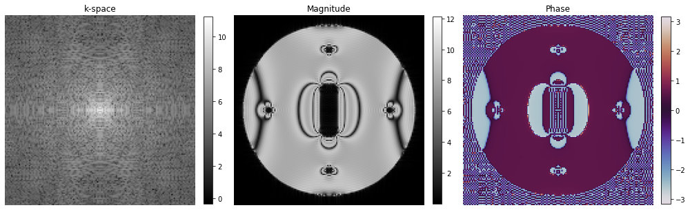
4. Reconstruct images#
[11]:
image = tf.signal.fftshift(tf.signal.ifft2d(tf.signal.ifftshift(k_space, axes=(0, 1))), axes=(0, 1)).numpy()
[12]:
# Show images
fig, axes = plt.subplots(1, 3, figsize=(14, 5))

kspace_plot = axes[0].imshow(np.log(np.abs(np.squeeze(k_space))), cmap="gray")
fig.colorbar(kspace_plot, ax=axes[0], fraction=0.045, pad=0.04)

abs_plot = axes[1].imshow(np.abs(np.squeeze(image)), cmap="gray")
fig.colorbar(abs_plot, ax=axes[1], fraction=0.045, pad=0.04)
phase_plot = axes[2].imshow(np.angle(np.squeeze(image)), cmap="twilight", vmin=-np.pi, vmax=np.pi)
fig.colorbar(phase_plot, ax=axes[2], fraction=0.045, pad=0.04)
[_.axis("off") for _ in axes]
[_.set_title(t) for _, t in zip(axes, ["k-space", "Magnitude", "Phase"])]
fig.tight_layout()