Turbulent Flow Trajectories#
This notebook demonstrates the usage of the TurbulentTrajectory class to generate particle trajectorie within a flow field containing Reynolds-stress tensors. The positional updates are performed according to the Langevin equation.
Imports#
[ ]:
!pip install cmrseq --index-url https://gitlab.ethz.ch/api/v4/projects/30300/packages/pypi/simple
[1]:
import sys
sys.path.append("../")
sys.path.insert(0, "../../")
sys.path.insert(0, "../../../cmrseq")

import os
os.environ["TF_CPP_MIN_LOG_LEVEL"] = "3"
os.environ['CUDA_VISIBLE_DEVICES'] = "3"

import tensorflow as tf
gpu = tf.config.get_visible_devices("GPU")
if gpu:
    tf.config.experimental.set_memory_growth(gpu[0], True)
[9]:
# 3rd Party dependencies
from pint import Quantity
import pyvista
import numpy as np
import matplotlib.pyplot as plt
from matplotlib import cm
from copy import deepcopy
from tqdm.notebook import tqdm
from time import perf_counter
from IPython.display import clear_output

# Project library cmrsim
import sys
import cmrsim
import cmrsim.utils.particle_properties as part_factory
Define positions of slice and refilling volume#
[3]:
dt = Quantity(0.01, "ms")
TR = Quantity(5, "ms")
num_TR = 50

# Define Reseeding slice parameters
seeding_slice_position = Quantity([0, 0.048, -0.045], "m")
seeding_slice_normal = np.array([1., 0., 0.])
seeding_slice_thickness = Quantity(50, "mm")
seeding_pixel_spacing = np.array((0.25e-3, 0.25e-3, 0.25e-3))  # resolution of seeding mesh, mm
seeding_slice_bb = Quantity([5, 5.1, 2], "cm")
seeding_particle_density = 3  # per 1/mm*3

# Define initial filling
initial_fill_normal = np.array([1., 0., 0.])
initial_fill_position = Quantity([-0.0005, 0., 0.], "m")
initial_fill_thickness = Quantity(50, "mm")
initial_fill_bounding_box = Quantity([25, 25, 25], "cm")
lookup_mesh_spacing = np.array((0.5e-3, 0.5e-3, 0.5e-3))  # resolution of lookup mesh, mm

steps_per_TR = int(np.round(TR/dt).m_as("dimensionless"))
Load UBend mesh#
First load the mesh and aling along z#
[4]:
# Load UBend Example
mesh = pyvista.read("../example_resources/sUbend_219_9.vtu")

# The velocity [m/s] is stored in the mesh as U1. In cmrsim all definitions are
# done in [ms] therefore we add the velocity field as scaled data to the mesh
mesh["velocity"] = Quantity(mesh["U"], "m/s").m_as("m/ms")
mesh.points = mesh.points[:, [2, 1, 0]]
mesh["velocity"] = mesh["velocity"][:, [2, 1, 0]]
mesh["RST"] = mesh["RST"][:, [5, 4, 2, 3, 1, 0]]
mesh["Reflectionmap"] = mesh["U"][:, 0] * 0 + 1  # in ms
tfreq = np.sqrt(np.sum(mesh["RST"][:, [0, 3, 5]], 1));
tfreq = tfreq / np.percentile(tfreq, 90) * 1000
mesh["Frequency"] = tfreq  # in Hz
Convert Reynolds stress tensor into cholesky decomposition#
[6]:
mesh["RST"] = mesh["RST"]  # m^2/s^2
# RST form xx xy xz yy yz zz

a11 = np.sqrt(np.clip(mesh["RST"][:, 0], 0, None) +
              np.min(np.abs(mesh["RST"][:, 0])))

a21 = mesh["RST"][:, 1] / a11
a22 = np.sqrt(np.clip(mesh["RST"][:, 3] - a21**2, 0, None) +
              np.min(np.abs(mesh["RST"][:, 3] - a21**2)))
a31 = mesh["RST"][:, 2] / a11
a32 = (mesh["RST"][:, 4] - a21 * a31) / a22
a33 = np.sqrt(np.clip(mesh["RST"][:, 5] - a31**2 - a32**2, 0, None))

# Cholesy form
mesh["chol"] = np.stack([a11, a21, a22, a31, a32, a33], axis=1) / 1000  # m/ms

global_mesh_offset = [0, 0.04, -0.05]
mesh.translate(global_mesh_offset, inplace=True)
mesh = mesh.cell_data_to_point_data()

# clip to restricted length to reduce mesh-size
mesh.clip(normal='-z', origin=[0., 0., -0.1], inplace=True)
print(np.percentile(np.sqrt(np.sum(mesh["RST"][:, [0, 3, 5]], 1)), 90))
0.8562077098606697
Instantiate RefillingFlowDataset#
[7]:
# setup initial fill dict
initial_fill_dict = {'slice_normal': initial_fill_normal,
                     'slice_position': initial_fill_position.m_as('m'),
                     'slice_thickness': initial_fill_thickness.m_as('m'),
                     'slice_bounding_box': initial_fill_bounding_box.m_as('m')}

# Setup flow dataset with seeding mesh information
particle_creation_fncs = {}

dataset = cmrsim.datasets.RefillingFlowDataset(mesh,
                                               particle_creation_callables=particle_creation_fncs,
                                               slice_position=seeding_slice_position.m_as("m"),
                                               slice_normal=seeding_slice_normal,
                                               slice_thickness=seeding_slice_thickness.m_as("m"),
                                               slice_bounding_box=seeding_slice_bb.m_as("m"),
                                               lookup_map_spacing=lookup_mesh_spacing,
                                               seeding_vol_spacing=seeding_pixel_spacing,
                                               field_list=[("velocity", 3), ("chol", 6), ("Frequency", 1), ("Reflectionmap", 1)])
mesh
Updated Mesh
/usr/local/lib/python3.11/dist-packages/pyvista/core/filters/data_set.py:3483: PyVistaDeprecationWarning: probe filter is deprecated and will be removed in a future version.
            Use sample filter instead.
            If using `mesh1.probe(mesh2)`, use `mesh2.sample(mesh1)`.

  warnings.warn(
Updated Slice Position
[7]:
| Header | Data Arrays | ||||||||||||||||||||||||||||||||||||||||||||||||||||||||||||||
|---|---|---|---|---|---|---|---|---|---|---|---|---|---|---|---|---|---|---|---|---|---|---|---|---|---|---|---|---|---|---|---|---|---|---|---|---|---|---|---|---|---|---|---|---|---|---|---|---|---|---|---|---|---|---|---|---|---|---|---|---|---|---|---|
|
|
Instantiate trajectory module#
[8]:
lookup_table_3d, map_dimensions = dataset.get_lookup_table()
trajectory_module = cmrsim.trajectory.TurbulentTrajectory(velocity_field=lookup_table_3d.astype(np.float32),
                                                          map_dimensions=map_dimensions.astype(np.float32),
                                                          additional_dimension_mapping=dataset.field_list[3:],
                                                          device="GPU:0")
Illustration 1 - Randomly seeded starts#
Run trajectory simulation#
This sections runs a manually defined loop of re-seeding particles at the inlet and moving updating their positions according to the turbulent flow field.
A subset of trajectories is saved during the loop for visualization purposes, therefore it is generally not required.
[10]:
# Allocate memory for saving the subset of trajectories
traj = []
npart = 250
tracking_inds = (np.round(np.random.uniform(0, 1, [npart, ]) * 20000).astype(np.int32)).tolist()
traj = np.zeros([npart, steps_per_TR * num_TR + 1, 3])

# Initial fill of particles
r, _ = dataset.initial_filling(particle_density=seeding_particle_density,
                               slice_dictionary=initial_fill_dict)

save_inds = list(range(np.shape(tracking_inds)[0]))
trajectory_module.warmup_step(particle_positions=r)

# Start particle tracking
traj[:, 0, :] = r[tracking_inds, :]
cur_dt = 1

# Refill once per repetition (TR) -> Loop over TRs
pbar = tqdm(range(num_TR), desc="Running Trajectory Sim", leave=True)
for tr in pbar:
    start = perf_counter()
    r_new = r
    pbar2 = tqdm(range(steps_per_TR), desc="Internal TR loop", leave=False)

    # Update particle positions during TR
    for _ in pbar2:
        r_new, _ = trajectory_module.increment_particles(r_new, dt.m_as("ms"))
        traj[save_inds, cur_dt, :] = r_new.numpy()[tracking_inds, :]
        cur_dt = cur_dt+1
    displacements = np.linalg.norm(r - r_new, axis=-1) * 1000
    mid = perf_counter()

    # Reseed particles
    r, _, in_tol = dataset(particle_density=seeding_particle_density,
                           residual_particle_pos=r_new.numpy(),
                           distance_tolerance=0.2,
                           reseed_threshold=1)

    # Keep track of the subset of particles for visualization
    removed_idx = []
    for ind, idx in zip(tracking_inds, range(len(tracking_inds))):
        new_ind = np.argwhere(in_tol[0] == ind)  # find its new index
        if new_ind.shape[0] == 0:  # check if particle is culled
            removed_idx.append(idx)
        else:  # if not, update index
            tracking_inds[idx] = new_ind[0][0]
    for ele in sorted(removed_idx, reverse=True):
        del tracking_inds[ele]
        del save_inds[ele]

    # Update trajectory modules with new particles
    n_new = dataset.n_new
    trajectory_module.turbulence_reseed_update(in_tol, new_particle_positions=r[-n_new:, :])

    # Format progressbar
    end = perf_counter()
    n_reused_particles = in_tol[0].shape[0] if in_tol is not None else 0
    pbar.set_postfix_str(
        f"Particles Reused: {n_reused_particles}/{r.shape[0]}  // "
        f" New vs. Drop: {n_new}/{dataset.n_drop}  // "
        f" Density: {dataset.mean_density: 1.3f}/mm^3 // "
        f" Durations: {mid - start:1.3f} | {end - mid:1.3f} // "
        f" Displacements: {np.median(displacements):1.1f},({np.percentile(displacements,97):1.2f},{np.percentile(displacements,3):1.2f}) mm"
    )
np.savez("illustration_1.npz", r_final=r, trajectory=traj)
clear_output()
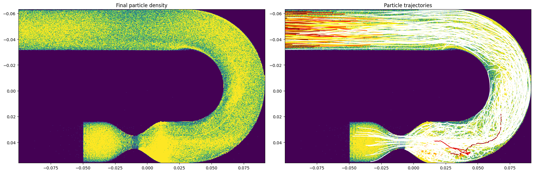
Plot results#
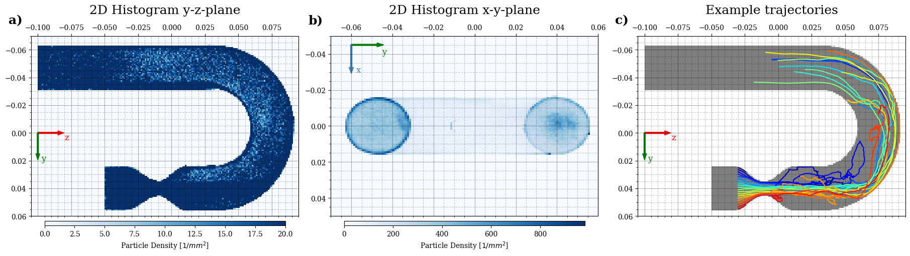
[12]:
%matplotlib inline
plt.close("all")
fig, axes = plt.subplots(1, 2, figsize=(18, 8))
A, xe, ye, _ = axes[0].hist2d(r[:, 1], r[:, 2], 600)
axes[0].clear()

for tr in range(traj.shape[0]):
    curtraj = traj[tr, :, :]
    trajlen = np.count_nonzero(np.sum(np.abs(curtraj), axis=1))
    axes[1].plot(np.trim_zeros(curtraj[:, 2]), np.trim_zeros(curtraj[:, 1]),
                 c=cm.hot(np.clip(trajlen/(steps_per_TR*num_TR), 0, 1)))

axes[0].imshow(A, vmax=5, extent=[ye.min(), ye.max(), xe.max(), xe.min()]);
axes[1].imshow(A, vmax=5, extent=[ye.min(), ye.max(), xe.max(), xe.min()]);
axes[0].set_title("Final particle density");
axes[1].set_title("Particle trajectories")
fig.tight_layout()
Plot 2D histogram#
Illustration 2 - Starting positions in a line#
This section used the same principle of particle tracking, however a specific set of particles at the inlet is tracked.
[14]:
# save initial fill for later only
r_initial, _ = dataset.initial_filling(particle_density=10, slice_dictionary=initial_fill_dict)
[15]:
lookup_table_3d, map_dimensions = dataset.get_lookup_table()
trajectory_module = cmrsim.trajectory.TurbulentTrajectory(velocity_field=lookup_table_3d.astype(np.float32),
                                                          map_dimensions=map_dimensions.astype(np.float32),
                                                          additional_dimension_mapping=dataset.field_list[3:],
                                                          device="GPU:0")
[17]:
steps = int(np.round(num_TR*TR/dt).m_as("dimensionless"))
r, properties, _ = dataset(seeding_particle_density)
npart = 20

# Seed particles in a straight line at the inlet before the stenosis
r = np.zeros([npart, 3], dtype=np.float32)
r[:, 2] = -3e-2
r[:, 0] = 0
center = 4e-2
cr = 1.5e-2
r[:, 1] = np.linspace(center - cr, center + cr, npart)

# Run particle tracking
pbar = tqdm(range(steps), desc="Running Trajectory Sim", leave=True)
traj = []
for step in pbar:
    r, _ = trajectory_module.increment_particles(r, dt.m_as("ms"))
    traj.append(r.numpy())
traj = np.asarray(traj)
np.savez("illustration_2.npz", r_final=r, trajectory=traj, r_initial=r_initial)
Create plot#
[20]:
%matplotlib inline
plt.close("all")
plt.rcParams['font.family'] = 'serif'

fig, axes = plt.subplots(1, 3, figsize=(18, 5), constrained_layout=True)
# density histogram z-y:
bins = [np.linspace(-0.07, 0.06, 131), np.linspace(-0.105, 0.095, 201)]
spacing = np.diff(bins[0])[0], np.diff(bins[1])[0]
print(spacing)
r_final = np.load("illustration_1.npz")["r_final"]
slice_indices = np.where(np.logical_or(r_final[:, 0] > 0.005, r_final[:, 0] < -0.005))
r_final[slice_indices, :] += np.array(((10, 1, 1)))
A, xe, ye, hist_artist = axes[0].hist2d(r_final[:, 2], r_final[:,1], bins=bins[::-1],
                                        density=False, cmap="Blues", vmax=20)

axes[0].grid(True, color="k", alpha=0.3)
axes[0].grid(which='minor', color='k', linestyle='--', alpha=0.2)
axes[0].minorticks_on()
fig.colorbar(hist_artist, location="bottom", orientation="horizontal", shrink=0.9, pad=0.001,
             fraction=0.9, aspect=50, label="Particle Density [$1/mm^2$]")
axes[0].text(-0.08, 0.005, "z", color="red", fontsize=12)
axes[0].arrow(x=-0.1, y=0, dx=.015, dy=0, color="red", width=0.001)
axes[0].text(-0.0975, 0.02, "y", color="green", fontsize=12)
axes[0].arrow(x=-0.1, y=0, dx=0, dy=.015, color="green", width=0.001)
axes[0].set_ylim(axes[0].get_ylim()[::-1]);
axes[0].tick_params(top=True, labeltop=True, bottom=False, labelbottom=False)

# density histogram y-x
bins = [np.linspace(-0.05, 0.05, 101), np.linspace(-0.07, 0.06, 131)]
spacing = np.diff(bins[0])[0], np.diff(bins[1])[0]
print(spacing)
r_final = np.load("illustration_1.npz")["r_final"]

A, xe, ye, hist_artist = axes[1].hist2d(r_final[:, 1], r_final[:, 0], bins=bins[::-1],
                                        density=False, cmap="Blues", vmax=None)
axes[1].grid(True, color="k", alpha=0.3)
axes[1].grid(which='minor', color='k', linestyle='--', alpha=0.2)
axes[1].minorticks_on()
fig.colorbar(hist_artist, location="bottom", orientation="horizontal", shrink=0.9, pad=0.001,
             fraction=0.9, aspect=50, label="Particle Density [$1/mm^2$]")
axes[1].text(-0.045, -0.04, "y", color="green", fontsize=12)
axes[1].arrow(x=-0.06, y=-0.045, dx=.0125, dy=0, color="green", width=0.00075)
axes[1].text(-0.0575, -0.03, "x", color="steelblue", fontsize=12)
axes[1].arrow(x=-0.06, y=-0.045, dx=0, dy=.0125, color="steelblue", width=0.00075)
axes[1].set_ylim(axes[1].get_ylim()[::-1]);
axes[1].tick_params(top=True, labeltop=True, bottom=False, labelbottom=False)

import skimage
r_initial = np.load("illustration_2.npz")["r_initial"]
traj = np.load("illustration_2.npz")["trajectory"]
axes[2].clear()

bins = [np.linspace(-0.07, 0.06, 131), np.linspace(-0.105, 0.095, 201)]
A, xe, ye, hist_artist = axes[2].hist2d(r_initial[:, 2], r_initial[:,1], bins=bins[::-1],
                                        density=False, cmap="gray_r", vmax=20, vmin=0, alpha=0.5)
axes[2].set_ylim(axes[2].get_ylim()[::-1]);
axes[2].tick_params(top=True, labeltop=True, bottom=False, labelbottom=False)

for tr in range(traj.shape[1]):
    curtraj = np.squeeze(traj[:,tr,:])
    axes[2].plot(curtraj[:,2],curtraj[:,1],c=cm.jet(np.clip(tr/traj.shape[1],0,1)))

axes[2].grid(True, color="k", alpha=0.3)
axes[2].grid(which='minor', color='k', linestyle='--', alpha=0.2)
axes[2].minorticks_on()
axes[2].text(-0.08, 0.005, "z", color="red", fontsize=12)
axes[2].arrow(x=-0.1, y=0, dx=.015, dy=0, color="red", width=0.001)
axes[2].text(-0.0975, 0.02, "y", color="green", fontsize=12)
axes[2].arrow(x=-0.1, y=0, dx=0, dy=.015, color="green", width=0.001)

axes[0].set_title("2D Histogram y-z-plane", pad=15, fontsize=18)
axes[1].set_title("2D Histogram x-y-plane", pad=15, fontsize=18)
axes[2].set_title("Example trajectories", pad=15, fontsize=18)

axes[0].text(-0.085, 1.12, 'a)', horizontalalignment='left', verticalalignment='top', transform=axes[0].transAxes, fontsize=18, fontweight="bold")
axes[1].text(-0.085, 1.12, 'b)', horizontalalignment='left', verticalalignment='top', transform=axes[1].transAxes, fontsize=18, fontweight="bold")
axes[2].text(-0.085, 1.12, 'c)', horizontalalignment='left', verticalalignment='top', transform=axes[2].transAxes, fontsize=18, fontweight="bold")
# fig.savefig("Figure6.tiff", dpi=750)
# fig.savefig("trajectory_turbulent_flow.png", dpi=200)
(0.0010000000000000009, 0.0010000000000000009)
(0.0010000000000000009, 0.0010000000000000009)
[20]:
Text(-0.085, 1.12, 'c)')