# OMatrix - Slice positioning in Sequences

Specifying a transformation for coordinates in the slice coordinate system / (Readout-Phase-SliceSelect) gradients directions is a common way to rotate the gradient waveforms and adjust the frequency offset of excitation pulses in MR sequences. In CMRseq this is captured in the cmrseq.OMatrix class. This notebook first show-cases the usage of this class on single gradient/rf blocks and subsequently shows how to register blocks within a cmrseq.Sequence instance with an OMatrix instance such that the gridded waveforms are transformed accordingly without mutating the block objects.

The OMatrix class

The OMatrix is instantiated from a RO-vector, a SS-vector and a scalar positional offset along the slice normal. When calling the apply() function, the point-wise definition of the gradient/rf waveforms are returned.

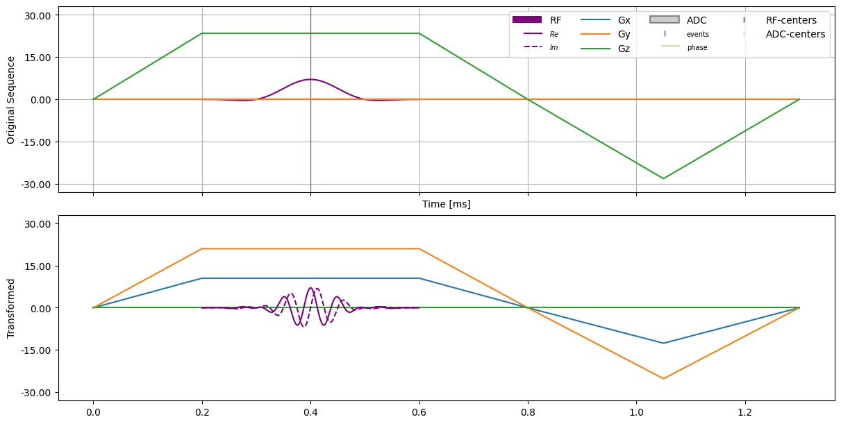
To show-case this, a slice-selective Sinc pulse with two trapezoidal gradients is initialized. The transformed rf and gradients are subsequently plotted.

import numpy as np
from pint import Quantity
import cmrseq

system_specs = cmrseq.SystemSpec(rf_raster_time=Quantity(1, "us"))
seq = cmrseq.seqdefs.excitation.slice_selective_sinc_pulse(system_specs,
                                                           slice_thickness=Quantity(10, "mm"),
                                                           flip_angle=Quantity(11, "degree"),
                                                           time_bandwidth_product=4,
                                                           pulse_duration=None,
                                                           slice_normal=np.array([0., 0., 1.]))

omatrix = cmrseq.OMatrix(Quantity(2., "cm"),
                         slice_normal=np.array([1., 2., 0.]),
                         readout_direction=np.array([0., 0., 1.]),
                         system_specs=system_specs)

# Upack the blocks to manually apply the OMatrix
trapezoid1, rf_pulse, trapezoid2 = seq[:]

# Passing in a Gradient block or its name returns a transformed definitions as (timepoints (t, ), waveform (3, t))
t1, gwf1 = omatrix.apply(trapezoid1)
t2, gwf2 = omatrix.apply(trapezoid2)

# To transform a RFPulse, the corresponding slice-selection gradient has to be specified. The complex waveform and time-points are return
rf_time, rf_waveform = omatrix.apply((rf_pulse, trapezoid1))

/usr/local/lib/python3.11/site-packages/tqdm/auto.py:21: TqdmWarning: IProgress not found. Please update jupyter and ipywidgets. See https://ipywidgets.readthedocs.io/en/stable/user_install.html
  from .autonotebook import tqdm as notebook_tqdm

Plotting the waveform yields the following figure:

import matplotlib.pyplot as plt
fig, axes = plt.subplots(2, 1, constrained_layout=True, figsize=(12, 6), sharex=True, sharey=True)

cmrseq.plotting.plot_sequence(seq, axes=[axes[0], ]*4, legend_position="upper right")
axes[0].set_ylabel("Original Sequence")

axes[1].plot(t1.m_as("ms"), gwf1[0].m_as("mT/m"), "C0"), axes[1].plot(t1.m_as("ms"), gwf1[1].m_as("mT/m"), "C1"), axes[1].plot(t1.m_as("ms"), gwf1[2].m_as("mT/m"), "C2");
axes[1].plot(t2.m_as("ms"), gwf2[0].m_as("mT/m"), "C0"), axes[1].plot(t2.m_as("ms"), gwf2[1].m_as("mT/m"), "C1"), axes[1].plot(t2.m_as("ms"), gwf2[2].m_as("mT/m"), "C2");
axes[1].plot(rf_time.m_as("ms"), rf_waveform.real.m_as("uT"), "-", color="purple"), axes[1].plot(rf_time, rf_waveform.imag, "--", color="purple");
axes[1].set_ylabel("Transformed")

The unit of the quantity is stripped when downcasting to ndarray.

Text(0, 0.5, 'Transformed')

Registering blocks in a Sequence

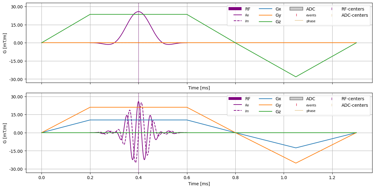
As the manual application for the orientation matrix is not very practical, the cmrseq.Sequence class offers a way to assign an OMatrix to given sequence blocks. When calling any of the *_to_grid() or combined_* functions, or even the property cmrseq.Sequence.gradients or cmrseq.Sequence.rf the transformed definitions are returned.

The block objects are however unchanged and contain the definition in slice-coordinates.

system_specs = cmrseq.SystemSpec(rf_raster_time=Quantity(1, "us"))
sequence = cmrseq.seqdefs.excitation.slice_selective_sinc_pulse(system_specs,
                                                                slice_thickness=Quantity(10, "mm"),
                                                                flip_angle=Quantity(40, "degree"),
                                                                time_bandwidth_product=4,
                                                                pulse_duration=None)

omatrix = cmrseq.OMatrix(Quantity(2., "cm"),
                         slice_normal=np.array([1., 2., 0.]),
                         readout_direction=np.array([0., 0., 1.]),
                         system_specs=system_specs)

# Plot the sequence without OMatrix
fig, axes = plt.subplots(2, 1, constrained_layout=True, figsize=(12, 6), sharex=True, sharey=True)
cmrseq.plotting.plot_sequence(sequence, axes=[axes[0], ]*4, legend_position="upper right")

# Register blocks. The gradients are passed as list of Gradient objects, and the rf-pulses are passed in as list of tuples (RFPulse, TrapezoidalGradient)
sequence.register_omatrix(omatrix,
                          gradients=[sequence[0], sequence[2]],
                          rf_pulses=[(sequence[1], sequence[0]),]
                         )

# Plot again with OMatrix
cmrseq.plotting.plot_sequence(sequence, axes=[axes[1], ]*4, legend_position="upper right")

import sys
sys.path.insert(0, "/scratch/jweine/cmrseq/")
# !export PYTHONPATH="/scratch/jweine/cmrseq/"