Introduction Part I - Sequence definition#
This notebook shows how to instantiate and modify sequences and how to use pint.Quantity objects. By composing a frequency encoded FID acqusition.
Imports#
[1]:
import sys
sys.path.insert(0, "../../..")
import cmrseq
import numpy as np
from pint import Quantity
import matplotlib.pyplot as plt
%matplotlib inline
System Limits definition#
First define system limits as a cmrseq.SystemSpec object. All quantities have a default value so they don’t have to be specified. for a complete list of inputs checkout the docstring.
The system specification object must be passed as argument to every constructor to allow validation against the system limits
[2]:
system_specs = cmrseq.SystemSpec(gamma=Quantity(42.575, "MHz/T"),
                                 grad_raster_time=Quantity(5, "us"),
                                 max_grad=Quantity(40, "mT/m"),
                                 max_slew=Quantity(120, "mT/m/ms"),
                                 rf_raster_time=Quantity(5, "us"),
                                 rf_peak_power=Quantity(30, "uT"),
                                 adc_raster_time=Quantity(0.1, "us"))
Instantiate Building Blocks:#
Sinc RF-pulse
readout pre-phaser (shortest duration for given k-space traverse)
readout gradient (duration matching the adc-block)
adc block
All building blocks contained in the cmrseq.bausteine module are implemented as subclasses of SequenceBaseBlocks, which implements common functions and properties that can be used to construct other building block as shown below. For a full list of building blocks check the API documentation.
As you can see below the TrapezoidalGradient class, implements multiple constructors using common combinations inputs to instantiate a corresponding gradient block.
[3]:
rf_excitation = cmrseq.bausteine.SincRFPulse(system_specs=system_specs,
                                             flip_angle=Quantity(np.pi/2, "rad"),
                                             duration=Quantity(1., "ms"),
                                             time_bandwidth_product=4,
                                             )


fov_x = Quantity(30, "cm")
kx_max = 2 / fov_x
prephaser_area = kx_max / system_specs.gamma
ro_prephaser = cmrseq.bausteine.TrapezoidalGradient.from_area(system_specs=system_specs,
                                                              area=prephaser_area,
                                                              orientation=np.array([-1., 0., 0.]))

adc_block = cmrseq.bausteine.SymmetricADC(system_specs=system_specs,
                                          num_samples=50,
                                          duration=Quantity(0.5, "ms"))

ro_gradient = cmrseq.bausteine.TrapezoidalGradient.from_fdur_area(system_specs=system_specs,
                                                                  orientation=np.array([1., 0., 0.]),
                                                                  flat_duration=adc_block.duration,
                                                                  area=prephaser_area*2)
[(b.tmin, b.tmax) for b in [rf_excitation, ro_prephaser, ro_gradient, adc_block]]
[3]:
[(0.0 <Unit('millisecond')>, 1.0 <Unit('millisecond')>),
 (0.0 <Unit('millisecond')>, 0.08 <Unit('millisecond')>),
 (0.0 <Unit('millisecond')>, 0.52 <Unit('millisecond')>),
 (0.0 <Unit('millisecond')>, 0.5 <Unit('millisecond')>)]
Compose Sequence#
Now shift the blocks to the correct time an compose the Sequence Object. The order in which the blocks are given to the Sequence does not matter on instantiation.
[4]:
ro_prephaser.shift(rf_excitation.tmax)
ro_gradient.shift(ro_prephaser.tmax)
adc_block.shift(ro_gradient.tmin + ro_gradient.rise_time)
sequence_obj = cmrseq.Sequence(building_blocks=[rf_excitation, ro_prephaser, ro_gradient, adc_block], system_specs=system_specs)
Visualize Sequence#
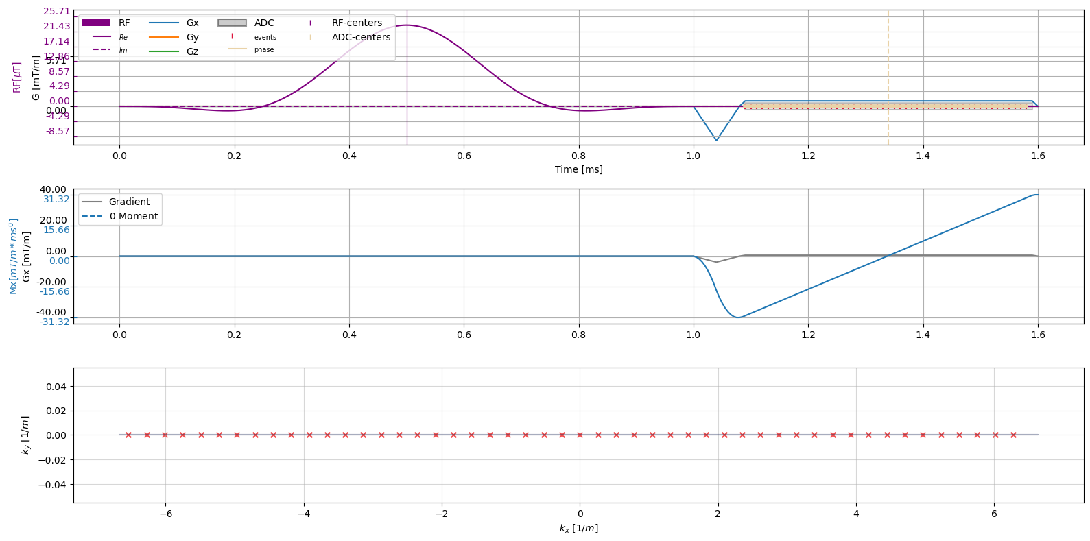
[5]:
fig, axes = plt.subplots(3, 1, figsize=(16, 8))
axes = axes.flatten()
axes[0].get_shared_x_axes().join(axes[0], axes[1])
cmrseq.plotting.plot_sequence(sequence_obj, axes=axes[0], n_yticks=15)
axes[0].set_ylim([-4.3889, 11.041])
fig.axes[-1].set_ylim([-10.9721, 27.6025])

cmrseq.plotting.plot_moment(sequence_obj, axes=[axes[1], axes[2], axes[2]])
axes[2].clear()
[a.remove() for a in fig.axes[-2:]]
cmrseq.plotting.plot_kspace_2d(sequence_obj, ax=axes[2], markersize=30)
fig.tight_layout()
/tmp/ipykernel_2564/3264493027.py:3: MatplotlibDeprecationWarning: The join function was deprecated in Matplotlib 3.6 and will be removed two minor releases later.
  axes[0].get_shared_x_axes().join(axes[0], axes[1])
