SE-M012-SSPEPI

This scenario aims at show-casing a typical workflow using the cmrseq package. The goal is to define a Spin Echo sequence with accellaration compensated diffusion weighting and a single shot EPI readout.

First we need to import a couple of python packages

import sys
sys.path.insert(0, "../../..")

import numpy as np
import matplotlib.pyplot as plt
%matplotlib inline
from pint import Quantity

import cmrseq

Defining system specifications

When working with cmrseq, for almost all functionality, it is necessary to define the system specifications as a cmrseq.SystemSpec object. All values are specified as pint.Quantity instances.

system_specs = cmrseq.SystemSpec(max_grad=Quantity(80, "mT/m"),
                                 max_slew=Quantity(200, "mT/m/ms"),
                                 grad_raster_time=Quantity(0.01, "ms"),
                                 adc_raster_time=Quantity(0.01, "ms"),
                                 rf_raster_time=Quantity(0.01, "ms"))

Search library SE-SSEPI

As a starting point for defining new sequences, it is a good idea to check the libary of composite sequence definitions in the cmrseq.seqdefs module. In there, you can find the function cmrseq.seqdefs.sequences.se_ssepi. The calling signature of this function is stated in the documentation as:

Parameters

- system_specs (SystemSpec) – SystemSpecification

- field_of_view (Quantity) – spatial extend in readout and phase encoding direction; shape = (2, )

- matrix_size (ndarray) – number of pixels in readout and phase encoding direction; shape = (2, )

- echo_time (Quantity) – Time at which the central k-space line is placed

- slice_thickness (Quantity) – Thickness of slice-selective excitation definitions

- slice_orientation (ndarray) – Slice normal of excitation slice

- pulse_duration (Quantity) – Duration of the excitation & refocusing pulses

- epi_slope_sampling (bool) – If yes the epi readout uses slope sampling - tbw_product (float) – Time-bandwidth product of the inc-Pulses used for excitation and refocus

- max_epi_duration (Quantity) - See documentation (cmrseq.seqdefs.readout.single_shot_epi) - epi_water_fat_shift (Quantity) - See documentation (cmrseq.seqdefs.readout.single_shot_epi) - partial_fourier_lines (int) – number of lines to skip before k-space center, allowing shorter echo times

- blip_direction (str) – from [“up”, “down”] defining the direction of phase-encoding kspace

Returns

sequence object

So let’s define the input parameters and call the function

fov = Quantity([230, 98], "mm")
resolution = Quantity([2.35, 2.35], "mm")
matrix_size = (fov / resolution).m.astype(int)
echo_time = Quantity(73, "ms")
slice_thickness = Quantity(10, "mm")
slice_orientation = np.array([0., 0., 1.])
pulse_duration = Quantity(2, "ms")
tbw_product = 4.
adc_duration = Quantity(0.4, "ms")

sequence = cmrseq.seqdefs.sequences.se_ssepi(system_specs, field_of_view=fov, matrix_size=matrix_size, echo_time=echo_time,
                                             slice_thickness=slice_thickness, slice_orientation=slice_orientation,
                                             pulse_duration=pulse_duration, epi_slope_sampling=True,
                                             tbw_product=tbw_product, epi_water_fat_shift="minimum")

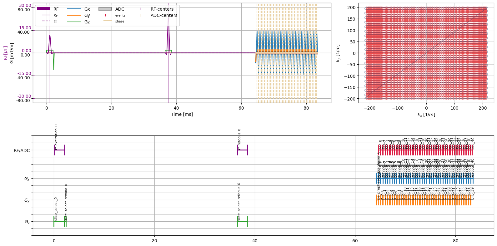
To get a graphical describtion of a sequence, using the cmrseq.plotting module offers some convient functionality:

# Instantiate matplotlib Figure:
figure = plt.figure(figsize=(16, 8))
axes = figure.subplot_mosaic("AAB;CCC")
axes = np.array([axes[k] for k in "ABC"])

# Use cmrseq plotting functionality:
cmrseq.plotting.plot_sequence(seq=sequence, axes=axes[0], plot_center_lines=True)
cmrseq.plotting.plot_kspace_2d(seq=sequence, k_axes=(0, 1), ax=axes[1])
cmrseq.plotting.plot_block_names(seq=sequence, axis=axes[2], fontsize=8)
figure.tight_layout()

Construct Diffusion Weighting

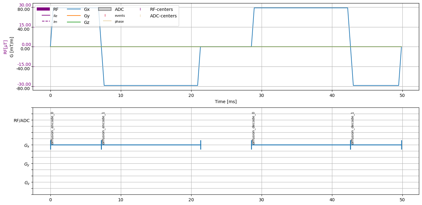
As you can see, the lower plot shows the names of building blocks contained in the sequence. All blocks have a unique name, which are set on adding a block to the sequence. Blocks have a user-defined name, which is augmented with a counter, to ensure unique-ness. A reference to a blocks can be obtained by calling sequence.get_block("block_name").

Now let’s create the diffusion encoding gradients and combine the sequences. Again, in the cmrseq.seqdefs.diffusion module we can find the the function m012, with the signature:

Parameters

- system_specs (SystemSpec)

- bvalue (Quantity) – B-Value in (s/mm^2), used to scale the waveform

- direction (ndarray) – (3, ) direction of gradient axis (is normalized internally)

- start_time (Quantity) – time offset before first lobe (to begin of rise)

- flip_decoding (bool) – In case of spin-echo sequences, the decoding lobes need to be inverted. If this argument is set to True the inversion is done internally.

Returns

- sequence object

After creating the sequence have a look at the result.

direction = np.array([1., 0., 0])
b_values = Quantity([450., ], "s/mm**2")

diffusion_weighting = cmrseq.seqdefs.diffusion.shortest_m012(system_specs=system_specs,
                                                             bvalues=b_values, direction=direction)

# Display the sequence
figure, axes = plt.subplots(2, 1, figsize=(16, 8))
cmrseq.plotting.plot_sequence(seq=diffusion_weighting, axes=axes[0], plot_center_lines=False)
cmrseq.plotting.plot_block_names(seq=diffusion_weighting, axis=axes[1], fontsize=8)

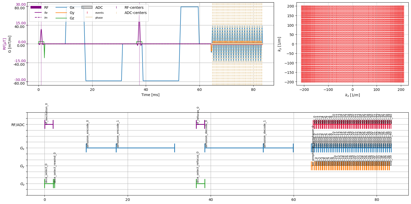
Combine Sequences

To combine the sequence and the diffusion weighting gradients, we now can use the sequence addition logic. Before adding the sequence we need to make sure, that the diffusion weighting gradients are shifted to the correct timing. Furthermore, since the sequence is a spin echo type we want to flip the decoding gradients.

# Calculate the required shift
refocus_end = sequence["slice_select_refocus_0"].tmax
decode_start = diffusion_weighting["diffusion_decode_0"].tmin
shift = system_specs.time_to_raster(refocus_end - decode_start, "grad")

# Shift and flip the diffusion gradients:
diffusion_weighting.shift_in_time(shift)
for block in diffusion_weighting.get_block(partial_string_match="diffusion_decode"):
    block.scale_gradients(-1)

# Add the sequences:
complete_sequence = sequence + diffusion_weighting

# Plot the Result:
figure = plt.figure(figsize=(16, 8))
axes = figure.subplot_mosaic("AAB;CCC")
axes = np.array([axes[k] for k in "ABC"])
cmrseq.plotting.plot_sequence(seq=complete_sequence, axes=axes[0], plot_center_lines=True)
cmrseq.plotting.plot_kspace_2d(seq=complete_sequence, k_axes=(0, 1), ax=axes[1], plot_raster_trajectory=False)
cmrseq.plotting.plot_block_names(seq=complete_sequence, axis=axes[2], fontsize=8)
figure.tight_layout()