Introduction II - Motion

This notebooks demonstrates the mechanism by which motion is integrated into the simulation.

In the course of this demonstration the distinction between two types of motion is made: 1. Motion during the readout 2. Motion between the shots

The reason for that is, that the way of passing motion information to the simulator differs for these to cases, while it can also be used jointly without any additional effort.

The examples are performed with the same Simulation-Definition as in the first notebook, while the phantom is a simple slice through three cylinders.

---

Setup the simulation and import packages

import sys
sys.path.append("../../")
sys.path.append("../../tests/")

import tensorflow as tf
physical_devices = tf.config.list_physical_devices('GPU')
if physical_devices:
    print("Available GPUS: \n\t", "\n\t".join([str(_) for _ in physical_devices]))
    tf.config.experimental.set_visible_devices(physical_devices[0], 'GPU')
    tf.config.experimental.set_memory_growth(physical_devices[0], True)

from collections import OrderedDict
import numpy as np
import math

import matplotlib.pyplot as plt
%matplotlib inline

import cmrsim
import phantoms

Available GPUS:
         PhysicalDevice(name='/physical_device:GPU:0', device_type='GPU')

from typing import Tuple

class ExampleSimulation(cmrsim.analytic.AnalyticSimulation):
    def build(self, matrix_size: Tuple[int, int] = (150, 150),
              field_of_view: Tuple[float, float] = (0.25, 0.3)):
        n_kx, n_ky = matrix_size

        # Encoding definition / To enable result comparisons, the noise is set to 0 here
        encoding_module = cmrsim.analytic.encoding.EPI(field_of_view=field_of_view, sampling_matrix_size=matrix_size,
                                                       read_out_duration=0.4, blip_duration=0.01, k_space_segments=n_ky,
                                                       absolute_noise_std=0.)
        # Signal module construction
        spinecho_module = cmrsim.analytic.contrast.SpinEcho(echo_time=50, repetition_time=10000)


        # Forward model composition
        forward_model = cmrsim.analytic.CompositeSignalModel(spinecho_module)

        # Reconstruction
        recon_module = cmrsim.reconstruction.Cartesian2D(sample_matrix_size=(n_kx, n_ky), padding=None)
        return forward_model, encoding_module, recon_module

---

Set up the Phantom

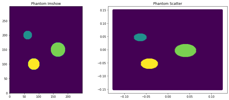
In the first step of generating a phantom for both motion types, a static 2D-gridded phantom is created. The motion is introduced, by modifying the positional vectors of the material points prior to handing it to the simulator.

phantom_dict, phantom_reference_map, coordinates = phantoms.define_cylinder_phantom((0.25, 0.3), (250, 300), background_value=0)
f, a = plt.subplots(1, 2, figsize=(12, 5))
a[0].imshow(phantom_reference_map, origin="lower")
a[1].scatter(coordinates[..., 0], coordinates[..., 1], c=np.abs(phantom_dict["M0"].reshape(-1)))
[_.set_title(t) for _, t in zip(a, ["Phantom Imshow", "Phantom Scatter"])]
f.tight_layout()

1. Motion during encoding

The strategy to incorporate motion, is to calculate the trajectory at the times defined as readout events by the encoding_module of the simulation.

These are then used to expand the #k-space-points axis of the r_vectors entry in the phantom dictionary:

# Instantiate simulator
simulator = ExampleSimulation(name='simulation_example', build_kwargs=dict(matrix_size=(100, 100), field_of_view=(0.25, 0.3)))

# Create static phantom
phantom_dict, phantom_reference_map, coordinates = phantoms.define_cylinder_phantom((0.25, 0.3), (250, 300), background_value=0)

non_trivial_material_point_indices = np.where(phantom_reference_map > 0.)
phantom_dict["r_vectors"] = phantom_dict["r_vectors"].reshape(300, 250, 3)

# Add flatten array and expand dims for repetition/kspace samples
flattened_phantom = {k:np.expand_dims(v[non_trivial_material_point_indices], axis=(1,2)) for k, v in phantom_dict.items()}
print("Phantom Definition: \t" , [f"{k}:{v.shape}" for k, v in flattened_phantom.items()])


# # Get readout event-times from the simulator
sampling_times = simulator.encoding_module.sampling_times.read_value().numpy()
print(f"Time range of read-out: [{np.amin(sampling_times)}, {np.amax(sampling_times)}] ms")

# Define a arbitrary function to calculate the new positions
# Example: constant velocity in x-direction
velocity = np.array([[2e-4, 0., 0.]])       # m/ms
delta_r = (velocity * sampling_times[:, np.newaxis])[np.newaxis]
print(f"Maximal displacement: {np.amax(delta_r, axis=(0, 1)) * 1e3} mm")

# Add displacement in x-direction over time to sample axis
r_vectors_new = np.tile(flattened_phantom["r_vectors"], [1, 1, sampling_times.size, 1])
r_vectors_new += delta_r.reshape(1, 1, -1, 3)

# Replace the vectors to the phantom
flattened_phantom['r_vectors'] = r_vectors_new
print("Shape of the old/new r-vectors:", coordinates.shape, r_vectors_new.shape)

Phantom Definition:      ['M0:(3883, 1, 1)', 'r_vectors:(3883, 1, 1, 3)', 'T1:(3883, 1, 1)', 'T2:(3883, 1, 1)', 'T2star:(3883, 1, 1)']
Time range of read-out: [0.0020000000949949026, 40.987998962402344] ms
Maximal displacement: [8.19759979 0.         0.        ] mm
Shape of the old/new r-vectors: (75000, 3) (3883, 1, 10000, 3)

Now feed the dictionary into the dataset class and run the simulation

dataset = cmrsim.datasets.AnalyticDataset(flattened_phantom, filter_inputs=False, expand_dimension=False)
simulated_images_1 = simulator(dataset, voxel_batch_size=750, execute_eager=False)

Run Simulation:         |XXXXXXXXXXXXXXX|3883/3883      |XXXXXXXXXXXXXXX|100/100

Visualize simulation results:

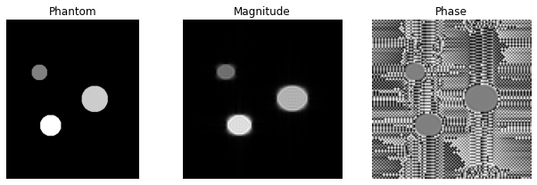
images_1 = np.squeeze(simulated_images_1)
magnitude, phase = np.abs(images_1), np.angle(images_1)
fig1, a = plt.subplots(1, 3)
a[0].imshow(np.abs(phantom_reference_map), cmap="gray", origin="lower")
a[1].imshow(magnitude, cmap="gray", origin="lower")
a[2].imshow(phase, cmap="gray", origin="lower")
a[0].set_ylabel("Motion during encoding")
[(_.axis("off"), _.set_title(t)) for _, t in zip(a, ["Phantom", "Magnitude", "Phase"])]
fig1.set_size_inches(9, 3), fig1.tight_layout()

(None, None)

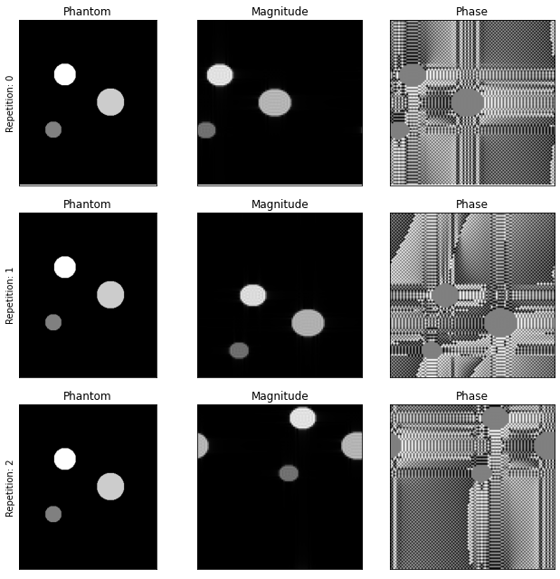
2. Motion in between repetitions

Similar to the expansion of the r-vectors array in the previous section, motion in-between repetitions can be introduced by changing the #repetitions axis of the position vectors.

# Instantiate simulator
simulator = ExampleSimulation(name='simulation_example', build_kwargs=dict(matrix_size=(100, 100), field_of_view=(0.25, 0.3)))

# Configure the simulation to acquire two repetitions with different echo-times
simulator.forward_model.spin_echo.TE.assign([20., 50., 100.])
simulator.forward_model.spin_echo.TR.assign([1e5, 1200., 900.])


# Create static phantom
phantom_dict, phantom_reference_map, coordinates = phantoms.define_cylinder_phantom((0.25, 0.3), (250, 300), background_value=0)
non_trivial_material_point_indices = np.where(phantom_reference_map > 0.)
phantom_dict["r_vectors"] = phantom_dict["r_vectors"].reshape(300, 250, 3)

# Add flatten array and expand dims for repetition/kspace samples
flattened_phantom = {k:np.expand_dims(v[non_trivial_material_point_indices], axis=(1,2)) for k, v in phantom_dict.items()}
print("Phantom Definition: \t" , [f"{k}:{v.shape}" for k, v in flattened_phantom.items()])


# Define a arbitrary function to calculate the new positions
r_vectors = flattened_phantom['r_vectors']
global_displacements = np.array([[-0.05, 0., 0.], [0., 0.05, 0.], [0.075, -0.075, 0.]]).reshape([1, 3, 1, 3])
r_vectors_new = r_vectors + global_displacements

# Replace the vectors to the phantom
flattened_phantom['r_vectors'] = r_vectors_new.astype(np.float32)

print("Shape of the old/new r-vectors:", r_vectors.shape, r_vectors_new.shape)

Phantom Definition:      ['M0:(3883, 1, 1)', 'r_vectors:(3883, 1, 1, 3)', 'T1:(3883, 1, 1)', 'T2:(3883, 1, 1)', 'T2star:(3883, 1, 1)']
Shape of the old/new r-vectors: (3883, 1, 1, 3) (3883, 3, 1, 3)

dataset = cmrsim.datasets.AnalyticDataset(flattened_phantom, filter_inputs=False, expand_dimension=False)
simulated_images = simulator(dataset, voxel_batch_size=5000, execute_eager=False)

Run Simulation:         |XXXXXXXXXXXXXXX|3883/3883      |XXXXXXXXXXXXXXX|100/100

f, axes = plt.subplots(3, 3)
images = np.squeeze(simulated_images)
print(images.shape)

for rep_idx, a, img in zip(range(3), axes, images):
    a[0].set_ylabel(f"Repetition: {rep_idx}")
    magnitude, phase = np.abs(img), np.angle(img)
    a[0].imshow(np.abs(phantom_reference_map), cmap="gray"), a[1].imshow(magnitude, cmap="gray"), a[2].imshow(phase, cmap="gray")
    [(_.set_xticks([]), _.set_yticks([]), _.set_title(t)) for _, t in zip(a, ["Phantom", "Magnitude", "Phase"])]
f.set_size_inches(9, 9), f.tight_layout()

(3, 100, 100)

(None, None)