Introduction I - Basic Functionality

This notebooks aims to show the basic concepts of the cmrsim frame work.

It is subdivided into the following subsections:

- Define the simulation - Define a digital phantom - Run the simulation - Auxiliary functions to save the simulation config

---

Import necessary python packages and cmrsim modules

For multi GPU environments, here the usage is limited to the first visibible device. In case no GPU is available CPU is used by default.

In case cmrsim is not installed in the virtual environment the repository root is added to the python path.

import sys
sys.path.append("../../tests/")

import tensorflow as tf
physical_devices = tf.config.list_physical_devices('GPU')
if physical_devices:
    print("Available GPUS: \n\t", "\n\t".join([str(_) for _ in physical_devices]))
    tf.config.experimental.set_visible_devices(physical_devices[0], 'GPU')
    tf.config.experimental.set_memory_growth(physical_devices[0], True)

from collections import OrderedDict
import numpy as np
import math

import matplotlib.pyplot as plt
%matplotlib inline

import cmrsim
import phantoms

Available GPUS:
         PhysicalDevice(name='/physical_device:GPU:0', device_type='GPU')

---

Define the simulation

As described in the readme and the documentation of the SimulationBase-class, there is the convenient way of subclassing the abstract Base-class. All subclasses need to implement the the _build method, where the composition of building blocks is performed. As the simulation parameters are defined as tf.Variables their values are easily modifyable at any time, even with graph execution.

The _build member-function must return a triple containing an instance of a subclassed EncodingBase module, a CompositeSignalModel (composing all signal operator building blocks) and an instance of a ReconBase module. If the simulation is meant to return the k-space signal, the third entry of the returned triple can be set to None.

The following ExampleSimulation is setup as a single shot (EPI) spin-echo, considering the T2* effects (TE-t, TE+t) with a simple inverse FFT as reconstruction.

from typing import Tuple
class ExampleSimulation(cmrsim.analytic.AnalyticSimulation):
    def build(self, matrix_size: Tuple[int, int] = (80, 100),
              field_of_view: Tuple[float, float] = (0.25, 0.3)):
        n_kx, n_ky = matrix_size

        # Encoding definition / To enable result comparisons, the noise is set to 0 here
        encoding_module = cmrsim.analytic.encoding.EPI(field_of_view=field_of_view, sampling_matrix_size=matrix_size,
                                                       read_out_duration=0.4, blip_duration=0.01, k_space_segments=n_ky,
                                                       absolute_noise_std=0.)
        # Signal module construction
        spinecho_module = cmrsim.analytic.contrast.SpinEcho(echo_time=50, repetition_time=10000)

        centered_times = tf.abs(encoding_module.get_sampling_times() - tf.reduce_max(encoding_module.get_sampling_times()) / 2)
        t2_star_module =  cmrsim.analytic.contrast.t2_star.StaticT2starDecay(centered_times)

        # Forward model composition
        forward_model = cmrsim.analytic.CompositeSignalModel(spinecho_module, t2_star_module)

        # Reconstruction
        recon_module = cmrsim.reconstruction.Cartesian2D(sample_matrix_size=(n_kx, n_ky), padding=None)
        return forward_model, encoding_module, recon_module

To run the simulation, a Simulator-object needs to be instantiated.

simulator = ExampleSimulation(name='simulation_example', build_kwargs=dict(matrix_size=(80, 100), field_of_view=(0.25, 0.3)))

Now display what the requirements for the digital phantoms are, i.e. which physical properties must each material point have assigned:

simulator.forward_model.required_quantities

('M0', 'T1', 'T2', 'T2star')

---

Define a digital phantom

In the following cell, a 2D object is constructed by loading a semantic mask (labels are integers) from the XCAT phantom.

The coordinates are assumed to lie on a regular-grid, therefore the utility of cmrsim.utils.coordinates is an easy way to calculate them.

As described in the README, the digital phantom is defined as OrderedDictionary of numpy arrays, where the keys are named after the entries of the required quantities. Furthermore, the assign_to_numerical_label_map is used to assign values according to the semantic label of the input map.

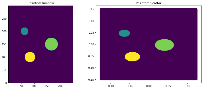
phantom_dict, phantom_reference_map, coordinates = phantoms.define_cylinder_phantom((0.25, 0.3), (250, 300), background_value=0)
f, a = plt.subplots(1, 2, figsize=(12, 5))
a[0].imshow(phantom_reference_map, origin="lower")
a[1].scatter(coordinates[..., 0], coordinates[..., 1], c=np.abs(phantom_dict["M0"].reshape(-1)))
[_.set_title(t) for _, t in zip(a, ["Phantom Imshow", "Phantom Scatter"])]
f.tight_layout()

To pass the phantom into the simulator, the dictionary is used to instantiate a costum tf.data.Dataset implemented in the BaseDataset class.

Note how the number of simulated material points (axis 1 of the printed shape) differs from what is shown in the progress-bar down below, while running the simulation. The reason for that is, on streaming the materialpoints during simulation, the entries with M0=0 are filtered out as they don’t yield signal. This is done to speed up simulations when the phantom is defined on a grid, that is likely to contain those 0-entries

for k, v in phantom_dict.items():
    if k != "r_vectors":
        phantom_dict[k] = v.reshape(-1)

print("Phantom Definition: \t" , [f"{k}:{v.shape}" for k, v in phantom_dict.items()])
dataset = cmrsim.datasets.AnalyticDataset(phantom_dict, filter_inputs=True, expand_dimension=True)

Phantom Definition:      ['M0:(75000,)', 'r_vectors:(75000, 3)', 'T1:(75000,)', 'T2:(75000,)', 'T2star:(75000,)']

---

Run the simulation

To start the simulation, use the __call__ function of the simulator instance {() - operator}.

For smaller images it might be beneficial to run the simulation in eager_mode, as building the computational Graph. Compare the times below, if a GPU is available eager exectuion should take 3-4 seconds while graph execution takes >5 seconds.

If the phatom gets larger (more material points), the time for building the Graph will get negligible, thus executing the simulation in eager mode is not advisable.

%time simulation_result = simulator(dataset, voxel_batch_size=20000, execute_eager=True)
%time simulation_result = simulator(dataset, voxel_batch_size=20000, execute_eager=False)

Run Simulation:         |XXXXXXXXXXXXXXX|3883/3883      |XXXXXXXXXXXXXXX|100/100 CPU times: total: 4.25 s
Wall time: 3.63 s
Run Simulation:         |XXXXXXXXXXXXXXX|3883/3883      |XXXXXXXXXXXXXXX|100/100 CPU times: total: 2.92 s
Wall time: 2.48 s

import ipywidgets as widgets

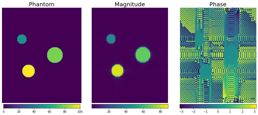
f, a = plt.subplots(1, 3, figsize=(13, 6))
magnitude_image = np.squeeze(np.abs(simulation_result))
phase_image = np.squeeze(np.angle(simulation_result))
img0 = a[0].imshow(phantom_reference_map, origin="lower")
img1 = a[1].imshow(magnitude_image, origin="lower")
img2 = a[2].imshow(phase_image, origin="lower")
[plt.colorbar(im, ax=ax, location="bottom", pad=0.01, shrink=0.9) for im, ax in zip([img0, img1, img2], a)]
[_.axis("off") for _ in a.flatten()]
[_.set_title(t, fontsize=20) for _, t in zip(a, ("Phantom", "Magnitude", "Phase"))]
f.tight_layout()

---

Auxilliary functions

1. Saving and Loading

The next cell shows how the simulation with all its configurations can be saved as tf.train.Checkpoint, and afterwards be restored from the checkpoint by calling the classmethod SimulationBase.from_checkpoint(...). To ensure that the parameters are equal, the simulation is redone and the results are compared.

import os

# Specify saving path
chkpt = './model_checkpoints/example_checkpoint'
os.makedirs(os.path.dirname(chkpt), exist_ok=True)

# Save simulation to checkpoint and delete old instance
simulator.save(checkpoint_path=chkpt)
del simulator

# construct new intance from checkpoint
new_simulator = ExampleSimulation.from_checkpoint(chkpt)

%time simulation_load_result = new_simulator(dataset, voxel_batch_size=5000, execute_eager=True)

print("If this is equal to zero, the simulated results are identical:\n\t Difference of simulated k-space ->",
      tf.reduce_sum(simulation_result - simulation_load_result))

Run Simulation:         |XXXXXXXXXXXXXXX|3883/3883      |XXXXXXXXXXXXXXX|100/100 CPU times: total: 1.98 s
Wall time: 1.37 s
If this is equal to zero, the simulated results are identical:
         Difference of simulated k-space -> tf.Tensor(0j, shape=(), dtype=complex64)

2. Manipulate Parameters

After instantitation of simulator instances, the variables contained in the submodules can be changed by directly accesing the tf.Variable.assign() method. To show if the results differ after setting different Echo-Times the simulated images are compared again:

new_simulator.forward_model.spin_echo.TE.assign([10,])  # in milliseconds
%time n = new_simulator(dataset, voxel_batch_size=5000)
print('Mean absolute difference for different TE:', tf.reduce_mean(tf.abs(simulation_load_result - n)))

new_simulator.forward_model.spin_echo.TE.assign([50,]) # in milliseconds
%time n = new_simulator(dataset, voxel_batch_size=5000)
print('Mean absolute difference for same TE:', tf.reduce_mean(tf.abs(simulation_load_result - n)))

Run Simulation:         |XXXXXXXXXXXXXXX|3883/3883      |XXXXXXXXXXXXXXX|100/100 CPU times: total: 3.97 s
Wall time: 2.37 s
Mean absolute difference for different TE: tf.Tensor(4.6015587, shape=(), dtype=float32)
Run Simulation:         |XXXXXXXXXXXXXXX|3883/3883      |XXXXXXXXXXXXXXX|100/100 CPU times: total: 3.16 s
Wall time: 2.38 s
Mean absolute difference for same TE: tf.Tensor(0.0, shape=(), dtype=float32)

3. Display summary as JSON

The SimulationBase class includes a functionality to create a report of the simulation configuration (aka submodule Variables) as dictionary. This dictionary can be used to generate a JSON string

import json
from IPython.display import JSON

summary_dict = new_simulator.configuration_summary
JSON(json.dumps(summary_dict))

C:\Users\Jonat\anaconda3\envs\tf29_pyvista\lib\site-packages\IPython\core\display.py:606: UserWarning: JSON expects JSONable dict or list, not JSON strings
  warnings.warn("JSON expects JSONable dict or list, not JSON strings")

<IPython.core.display.JSON object>