Two Water Tanks
Physical system
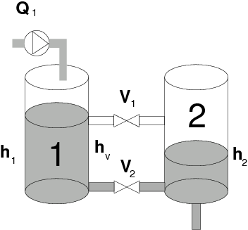
The two-tanks systems consists of two tanks which are connected by
two valves. Liquid inflow Q1 to the first tank is governed by
a pump and there are two interconnections between the tanks:
- Through Valve 1, which is always fully open.
The liquid flows through this valve if
h1 > hv.
- Through Valve 2, which can be either fully open (
V2=1),
or fully closed (V2=0).
In addition, there is a permanent leak from tank 2. The system has two
manipulated variables:
- Liquid inflow
Q1 which can change continuously.
- Position of Valve 2 which can be either fully open (
V2=1),
or fully closed (V2=0). No other positions are allowed.
The system is subject to constraints on liquid inflow and heights of liquid levels in both
tanks. The two-tanks system shows clear characteristics of hybrid systems.
First, the dynamics changes depending on current operating conditions (e.g. there
is a direct flow from tank 1 to tank 2 through Valve 1 if level in the
first tank is above certain level), and secondly, some system inputs are in fact
on-off switches, such as Valve 2.
Control objectives
The aim is to design a controller which is able to stabilize
liquid level in the second tank at the given reference point h2 = 0.2 m.
The controller can manipulate liquid inflow Q1 continuously in
range of 0 <= Q1 <= 1 and position
of Valve 2, which can only take boolean values 0 or 1.
The controller must cope with different constraints and have good
regulation performance.
Modelling in HYSDEL
SYSTEM twotanks {
  INTERFACE {
    STATE {
      REAL h1 [0, 0.62];  /* level in 1st tank */
      REAL h2 [0, 0.62];   /* level in 2nd tank */
    }
    INPUT {
      REAL q1 [0, 1];     /* liquid inflow */
      BOOL V2;            /* position of Valve 2 */
    }
    OUTPUT {
      REAL y;             /* output = h2 */
    }
    PARAMETER {
      REAL dT = 10;       /* sampling time */
      REAL hv = 0.3;      /* height of Valve 1 */
      REAL s = 10e-6;     /* scross-section of valves */
      REAL hmax = 0.62;   /* maximum height of liquid */
      REAL g = 9.81;
      REAL F = 0.0143/dT; /* area of each tank */
      REAL q_in = 0.1e-3; /* maximum liquid inflow */
      REAL k1 = s*sqrt(2*g/(hmax-hv));
      REAL k2 = s*sqrt(2*g/hmax);
    }
  }
  IMPLEMENTATION {
    AUX {
      /* auxiliary variables */
      REAL z1_1, z2_1, z3_1, z4_1;
      REAL z1_2, z2_2, z3_2, z4_2;
      BOOL above;
    }
    AD {
      above = h1 >= hv;    /* d1 will be true iff h1 >= hv */
    }
    DA {
    z1_1 = {
      /* h1>=hv and V2 open */
      IF (above & V2) THEN
        (1-k1/F)*h1 - k2/F*h2 + hv/F*k1
      ELSE
        0
      };

      z1_2 = {
        /* h1>=hv and V2 open */
        IF (above & V2) THEN
          (k1+k2)/F*h1 +  (1-k2/F)*h2 - hv/F*k1
        ELSE
          0
      };

      z2_1 = {
        /* h1 <=hv and V2 open */
        IF (~above & V2) THEN
          (1-k2/F)*h1
        ELSE
          0
      };

      z2_2 = {
        /* h1 < hv and V2 open */
        IF (~above & V2) THEN
          k2/F*h1 + (1-k2/F)*h2
        ELSE
          0
      };

      z3_1 = {
        /* h1>=hv and V2 closed */
        IF (above & ~V2) THEN
          (1-k1/F)*h1 + k1/F*hv
        ELSE
          0
      };

      z3_2 = {
        /* h1>=hv and V2 closed */
        IF (above & ~V2) THEN
          k1/F*h1 + (1-k2/F)*h2 - k1/F*hv
        ELSE
          0
      };

      z4_1 = {
        /* h1<=hv and V2 closed */
        IF (~above & ~V2) THEN
          h1
        ELSE
          0
      };

      z4_2 = {
        /* h1<=hv and V2 closed */
        IF (~above & ~V2) THEN
          1-k2/F
        ELSE
          0
      };
    }
    CONTINUOUS {
      /* state update equations */

      /* h1(k+1) = ... */
      h1 = z1_1 + z2_1 + z3_1 + z4_1 + q_in/F*q1;

      /* h2(k+1) = ... */
      h2 = z1_2 + z2_2 + z3_2 + z4_2;
    }
    OUTPUT {
      /* output is just h2 */
      y = h2;
    }
    MUST {
      /* level in tank 2 must be below level in tank 1 */
      h2 <= h1;
    }
  }
}
Controller design in MPT
In order to design a model-based controller with MPT, we first
need to define model of the dynamical system. We can do that
by importing the HYSDEL model and converting it into an
equivalent Piecewise-Affine (PWA) model:
>> Ts = 10;                               % sampling time
>> model = mpt_sys('twotanks.hys', Ts);
The command mpt_sys will read description of
the system stored in file twotanks.hys and convert
it into an PWA model.
Second step is to define system constraints:
>> ymax = 0.62;          % maximum  height of liquid in 2nd tank
>> ymin = 0;            % minimum height of liquid in 2nd tank
>> qmax = 1;            % maximum inflow (manipulated variable Q1)
>> qmin = 0;            % minimum inflow (manipulated variable Q1)
>> v2max = 1;           % maximum value for Valve 2
>> v2min = 0;           % minimum value for Valve 2

>> model.ymax = ymax;
>> model.ymin = ymin;
>> model.umax = [qmax; v2max];
>> model.umin = [qmin; v2min];
Now we can define the optimization problem. Our objective is to
obtain a controller which stabilizes liquid level in the second
tank at h2_ref = 0.2. Our controller will predict
system behavior 3 sampling times into the future, choosing such
control actions which minimize the difference between the predicted
output and our given reference:
>> problem.N = 3;             % prediction horizon
>> problem.yref = 0.2;        % reference value for outputs
>> problem.norm = 1;          % cost function based on 1-norms
>> problem.Qy = 100;          % cost which penalizes (y-yref)
>> problem.Q = zeros(2);      % zero cost on states
>> problem.R = 1e-3*eye(2);   % cost which penalizes usage of inputs
Once the model and the problem are given, the controller can
be obtained by
>> controller = mpt_control(model, problem);
Results and simulations
For the parameters specified above, the controller consists of
136 regions which can be plotted using
>> plot(controller)
The controller can now be either used for simulations, or
exported to C-code for embeding into the real application. To
simulate the closed-loop system from a given starting conditions,
one would use
>> x0 = [0.5; 0];     % initial conditions h1=0.5m, h2=0
>> Nsim = 60;         % number of simulation steps
>> simplot(controller, x0, Nsim)
Of course you can choose any initial conditions which the controller covers.
The function simplot also allows you to choose
such initial points on mouse-click if the initial state x0
is not provided:
>> simplot(controller);
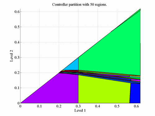
The controller can be further simplified to reduced number of regions.
The command to do such a simplification is as follows:
>> simple_controller = mpt_simplify(controller);
The simplification is based on merging regions which have the same
control law, which guarantees that the simplified controller will
maintain fullfilment of the same control objectives as the original
controller does. The simplified controller consists of 50 regions
and is depicted on the figure below.