A Gas Actuated Hopping Machine

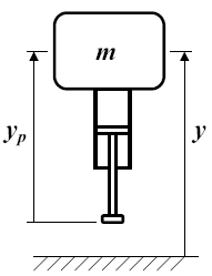
Physical system

The gas actuated hopping machine is driven by a penumatic actuator, with the location of the piston relative to the mass under no external loading defined as yp. After contact occurs with the ground with y<=yp, the upward force on the mass from actuator can be approximated by a linear spring with F = k(yp-y); where k is the spring constant. The position yp can be viewed as the unstretched spring length and it can be easily changed by pumping air into or out of either side of the cylinder. 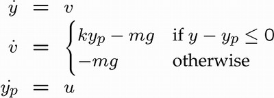The equations of motion for the mass are

The system is subject to constraints on maximal and minimal piston position yp, as well as on the control input u. Behavior of the system shows clear hybrid characteristics, since the force F takes non-zero values if the machine hits the ground, otherwise the external force due to the piston has no effect on the machine movement.

Control objectives

The control objective is to make the machine hopping, reaching a given jump height. Moreover, we would like the controller to manipulate the external input u(t) in such a way, such that the machine is driven to a respective reference as quickly as possibly, i.e. in minimum time.

Modelling in HYSDEL

A simple Euler approximation can be used to discretize the equations of motions. Then the following HYSDEL model describes behavior of the hopping machine under different operating conditions:

SYSTEM hopper {
INTERFACE {
    STATE {
        REAL y [0, 30];         /* mass height */
        REAL speed [-30, 30];   /* mass speed */
        REAL yp [0, 5];         /* piston position */
    }
    INPUT {
        REAL u [-20, 20];       /* air inflow */
    }
    OUTPUT {
        REAL height;            /* output = mass height */
    }
    PARAMETER {
        REAL dt = 0.1;      /* sampling time */
        REAL k = 500;       /* spring constant */
        REAL m = 1;         /* mass */
        REAL g = 386 * dt;  /* acceleration due to gravity */
    }
}
IMPLEMENTATION {
    AUX {
        /* auxiliary variables */
        BOOL groundhit;     
        REAL aux_speed;
    }
    AD {
        /* the 'groundhit' variable will be true iff we hit the ground */
        groundhit = y - yp <= 0;
    }
    DA {
        aux_speed = { 
            IF groundhit THEN 
                /* when the machine hits the ground, additional
                   upwards force is generated due to the piston */
                dt*(k*yp - g) 
            ELSE 
                /* while in the air, only gravity affects the motion */    
                -dt*g + speed 
        };
    }
    CONTINUOUS {
        /* state update equations */
        y = dt*speed + y;
        speed = aux_speed;
        yp = dt*u + yp;
    }
    OUTPUT {
        height = y;
    }
  }
}

Controller design in MPT

In order to design a model-based controller with MPT, we first need to define model of the dynamical system. We can do that by importing the HYSDEL model and converting it into an equivalent Piecewise-Affine (PWA) model:

>> Ts = 0.1;                            % sampling time
>> model = mpt_sys('hopper.hys', Ts);

The command mpt_sys will read description of the system stored in file hopper.hys and convert it into an PWA model. Second step is to define system constraints:

>> model.ymax = 30;    % maximum height of mass
>> model.ymin = 0;    % minimum height of mass
>> model.umax = 20;    % maximum allowed airflow to piston
>> model.umin = -20;   % minimum allowed airflow to piston

Now we can define the optimization problem. Our objective is to design a controller which drives the mass into a given reference position in minimum time. Therefore the first step is to define a minimum-time control problem:

>> problem.subopt_lev = 1;       % use minimum-time strategy
>> problem.N = Inf;              % for minimum-time problems
>> problem.norm = 2;             % use quadratic cost function
>> problem.Q = diag([0 0.1 0]);  % penalty on states
>> problem.R = 1;                % penalty on input

In addition, we need to specify a target region, to which system states will be driven. Such region in our case is given by following inequalities:

19.8 <=  y(k) <= 20.2
  -5 <=  v(k) <= 5
   0 <= yp(k) <= 5

The first inequality says that the mass position should reach a range between 19.8 and 20.2 inches. Second term specifies that once the mass is at a given reference, it's speed should not exceed +/- 5 inches/sec. Finally, the third inequality says that the piston position should not exceed given bounds. The inequalities above can be translated into a polytope:

>> H = [eye(3); -eye(3)];
>> K = [20.2; 5; 5;  -19.8; 5; 0];
>> problem.Tset = polytope(H, K);    % target set

Once the model and the problem are given, the controller can be obtained by

>> controller = mpt_control(model, problem);

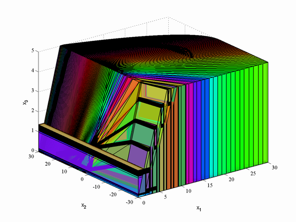
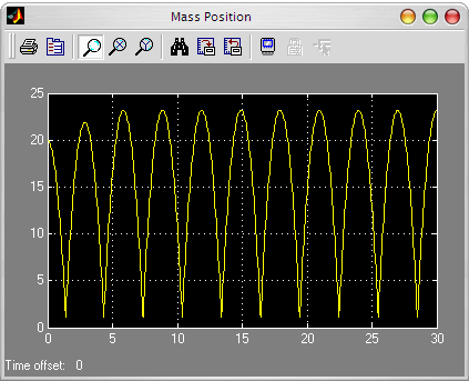
Results and simulations

For the parameters specified above, the controller consists of 326 regions in 3D state-space, which can be plotted using

>> plot(controller)

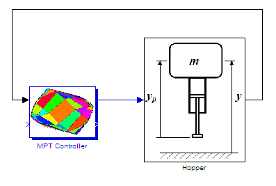
The controller can now be either used for simulations, or exported to C-code for embeding into the real application. In this demonstration we simulate the closed-loop system on a non-linear model of the hopping machine in Simulink:

which leads the following closed-loop response: