Analytic Simulations#
Note
Notebooks demonstrating the content described below can be found by navigating to Examples in the navigation bar at the top of the page
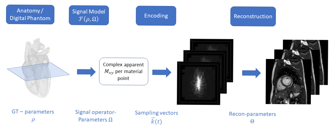
As an overview the concept of analytic CMRsim simulation can be described by following sub-sections:
Components 1-4 are composed into a Simulator object that uses component 1 as input. Detailed explanations are given in following sections. Explanation along code examples can be found in the introductory notebooks also presented on this page.
0. Input Shape Explanations#
As mentioned in the section input defintions, the input to analytic simulations include axes that might seem unintuitive. Therefore, more detailed explanation is given as:
- points:
Number of material points constituting the object
- repetitions:
In case the simulation incorporates multiple images with different values of e.g. TE or TR, all images are simulated in one go. To ensure, that the shape is matching during simulation, all arrays are specified in that shape. If the property does not change between acquisitions the dimension the #repetitions axis is trivially set to 1, and the simulation is expected to broadcast the input accordingly.
- k-space-samples:
This axis is meant to facilitate, changes of the properties during encoding. The most use-case would be motion/displacement over the course of encoding as demonstrated in Introductiin II. The sampling-time associated which each k-space point is defined by the encoding module. If only the position changes, the simulation modules are expected to broadcast the other inputs accordingly.
1. The Signal Model#
The complete signal model is represented by a cmrsim.analytic.CompositeSignalModel object,
which contains a collection of operator-modules (i.e. objects of
cmrsim.analytic.contrast.BaseSignalModel subclasses). Consecutively calling the operator-modules
corresponds to the formulation of calculating the transverse magnetization by applying the
signal operators (e.g. exponential decay due to diffusion) to the initial magnetization per particle.
Parameters of operators are defined as members of the module (as tf.Variable), while particle properties are given as input argument to the operator call. All operators __call__ functions take the **kwargs argument alongside the required quantities. So passing the dictionary unpacked digital phantom is valid for all operators as long all required quantities are present. The following example illustrates this mechanism:
# Instantiate the operator with TE=20ms and TR=5s
spinecho_operator = cmrsim.analytic.contrast.SpinEcho(echo_time=20., repetition_time=5000.)

# Create a dummy phantom with a single particle:
dummy_phantom = dict([
        M0=np.ones([1, 1, 1], dtype=np.complex64),
        T1=np.ones([1, 1, 1], dtype=np.float64) * 1000,
        T2=np.ones([1, 1, 1], dtype=np.float64) * 250,
    ])

# Call operator
result = spinecho_operator(signal_tensor=dummy_phantom["M0"], **dummy_phantom)
>>> result.shape: (1, 1, 1)
Composing a signal model is done by passing an ordered sequence of operators as input to a composite signal model. Calling the composite signal model, evaluates all operators while preserving the input order (corresponding to a pipe-and-filter pattern). The repetition and sampling axes can be expanded by the signal operator modules as demonstrated example below:
# Instantiate an SE operator with two sets of TE and TR
spinecho_operator = cmrsim.analytic.contrast.SpinEcho(echo_time=[20., 50.],
                                                      repetition_time=[5000., 5000.])

# Instantiate a T2*-weighting (relative to echo time)
# Note: the sampling times are just a placeholder to illustrate the shapes
t2star_operator = cmrsim.analytic.contrast.StaticT2starDecay(sampling_times=np.linspace(-100, 100, 200)))

# Create a dummy phantom with a single particle:
dummy_phantom = dict([
        M0=np.ones([1, 1, 1], dtype=np.complex64),
        T1=np.ones([1, 1, 1], dtype=np.float64) * 1000,
        T2=np.ones([1, 1, 1], dtype=np.float64) * 250,
        T2star=np.ones([1, 1, 1], dtype=np.float64) * 35
    ])

# Compose the signal model
signal_model = cmrsim.analytic.CompositeSignalModel([spinecho_operator, t2star_operator])

# Call operator
result = signal_model(signal_tensor=dummy_phantom["M0"], **dummy_phantom)
>>> result.shape: (1, 2, 200)
2. The Encoding Module#
The encoding module performs evaluation of the Fourier-integration over the entire volume. To
facilitate the scalability of the phantom, this integration is performed as an accumulation of
signal per k-space point. The base implementation of the encoding operator
(cmrsim.analytic.encoding.BaseSampling) has an abstract method to calculate the
k-space-trajectory, but already implements the batched evaluation functionality. This way it
is easy to implement specific sampling patterns without the need to touch the rest of the code.
Additionally, the cmrsim.analytic.encoding.GenericEncoding class uses a cmrseq sequence
to construct the sampling pattern, such that translation from sequence definition to simulation
is seamless. The following example illustrates the process of implementing your own encoding module:
from cmrsim.analytic.encoding import BaseSampling

# Subclass the BaseSampling class
class MyNewEncoder(BaseSampling):
    def _calculate_trajectory(self):
        # Do some calculations to generate k-space-vectors and sampling times
        # of shape (N, 3), (N)
        return k_vectors, sampling_times

# Instantiate an encoder
# Note: adding noise is performed further downstream, where the number of different
#       Noise-levels can be specified on instantiation:
encoding_operator = MyNewEncoder(..., absolute_noise_std=[0, 0.1])

# Assume that signal_tensor is one batch of output of the composite signal model
# Having a shape of (P, R, N)
k_space_batch = encoding_operator(signal_tensor)
k_space_with_noise = encoding_operator.add_noise(k_space_batch)
# Note the expansion of the second to last axis by the number of noise-levels
k_space_batch.shape, k_space_with_noise.shape,
>>> (r, 1, N), (r, 2, N)
3. The AnalyticSimulation class#
To reduce boiler plate code of setting up the batched input stream and calling the previously
described components, the cmrsim.analytic.AnalyticSimulation bundles these functionlities.
Furthermore the simulator-object allows saving, exporting as JSON and some other functions.
There are two options of instantiating a Simulator object as shown below: Note: In both cases no reconstruction is specified, in which case the k-space is returned.
# Assume the encoding model to be defined as shown above
signal_model = cmrsim.analytic.CompositeSignalModel([...])
encoding_operator = MyNewEncoder(..., absolute_noise_std=[0, 0.1])

simulator = cmrsim.analytic.AnalyticSimulation(
                        building_blocks=(signal_model, encoding_operator, None)
                )
This is especially useful for parameterized simulation definitions (e.g. comparative simulation experiments)
class MyNewSimulation(cmrsim.analytic.AnalyticSimulation):
    def build(self, **my_defined_inputs):
        signal_model = cmrsim.analytic.CompositeSignalModel([...])
        encoding_operator = MyNewEncoder(..., absolute_noise_std=[0, 0.1])
        reconstruction_module = None
        return signal_model, encoding_operator, reconstruction_module

simulator = MyNewSimulation(build_kwargs=my_defined_inputs)
Batching and asserting correct shapes is achieved by wrapping the phantom with a cmrsim dataset. To evaluate the simulation just call the simulator object with the given input dataset.
dummy_phantom = dict([
        ...
    ])
dataset = cmrsim.dataset.AnalyticDataset(dummy_phantom)
k_space = simulator(dataset)
4. [Optional] The Reconstruction Module#
The Reconstruction module has to be choosen according to the encoding in the simulation. As the k-space-sample axis is flatten, the user has to check if encoding and recon match (e.g. 2D-EPI & iFFT). As it may be desirable to not include the reconstruction into the Simulation call, the specification of the recon module is optional. If a Subclassed module of BaseRecon is specified as recon module, the returned tensor contains data in image space. As no Modules follow after reconstruction there are no restrictions are enforced for the output shape of the reconstructed images.