MPT 2.5 Changelog

Hybrid Identification Toolbox included (pre release 0.95)

The Hybrid Identification Toolbox (HIT) by Giancarlo Ferrari-Trecate can solve two types of problems:

Regression problem: reconstruct a PWA map from noisy samples. In this case, one is not dealing with a dynamical system (with inputs and outputs) but just with a static map that is sampled. HIT gives you back a data-based PWA approximation of the map (see the examples ex_approx_1d.m and ex_cake1.m - the second example shows how to approximate discontinuous PWA maps). The approximation has idmodes.s modes (in HITs jargon, a "mode" is an affine hyperplane + the region where is valid).
Identification problem: reconstruct a PWARX hybrid system from noisy inputs and outputs (see for instance ex_pwarx_2d_3modes.m). PWARX systems are multi-input/single-output descriptions of hybrid systems. Thus no state appears. But they can be re-written as PWA system pretty much the same way ARX models can be re-written as linear systems in the state-space form.

The PWARX systems used in the HIT toolbox are of the form

y(k)=idmodes.par{i}* [x(k)' 1]' if x(k) \in \idmodes.regions(i)

where x(k)=[y(k-1) ... y(k-na) u'(k-1) ... u'(k-nb)]' is the vector of regressors and the integers na and nb are the system order. If you want to write a PWARX model in the PWA form you have to interpret x(k) as a state, y(k) as an output and find the matrices A_i, b_i, f_i, C_i, D_i, g_i that given a sequence u(k) produce the same output of the PWARX model.

The Hybrid Identification Toolbox can be found in the mpt/hit directory of your MPT installation.

Required software: MATLAB 6.5 (or higher).

Ellipsoidal Toolbox included

The Ellipsoidal Toolbox by Alex Kurzhanskiy is a standalone set of easy-to-use configurable MATLAB routines to perform operations with ellipsoids and hyperplanes of arbitrary dimensions. It computes the external and internal ellipsoidal approximations of geometric (Minkowski) sums and differences of ellipsoids, intersections of ellipsoids and intersections of ellipsoids with halfspaces and polytopes; distances between ellipsoids, between ellipsoids and hyperplanes, between ellipsoids and polytopes; and projections onto given subspaces.

Ellipsoidal methods are used to compute forward and backward reach sets of continuous- and discrete-time piecewise affine systems. Forward and backward reach sets can be also computed for continuous-time piece-wise linear systems with disturbances. It can be verified if computed reach sets intersect with given ellipsoids, hyperplanes, or polytopes.

The toolbox provides efficient plotting routines for ellipsoids, hyperplanes and reach sets.

You will find the Ellipsoidal Toolbox in the mpt/ellipsoids directory of your MPT installation. To start, have a look at ell_demo1, ell_demo2 and ell_demo3 demos.

Required software: MATLAB 6.5 (or higher).

Latest release of YALMIP included

YALMIP by Johan Löfberg is a MATLAB toolbox for rapid prototyping of optimization problems. The package initially focused on semi-definite programming, but the latest release extends this scope significantly. YALMIP can now be used for:

convex linear, quadratic, second order cone and semidefinite programming.
non-convex quadratic and semidefinite programming (local & global).
mixed integer conic programming.
multi-parametric parametric programming.
geometric programming.

The latest relase of YALMIP has improved integration between YALMIP and MPT. YALMIP adds a layer above the algorithms in MPT, allowing you to, e.g., symbolically define and solve multi-parametric linear programs with binary variables, and easily construct dynamic programming based algorithms. Additionally, YALMIP adds support for working with piecewise affine functions in a symbolic fashion. Read more about this in the YALMIP manual (type open('yalmip.htm') in MATLAB.)

YALMIP can be found in the mpt/yalmip directory of your installation. You can learn more about YALMIP by looking on its demos; just run yalmipdemo and enjoy.

Optimal control of PWA systems with quadratic stage cost

MPT 2.5 introduces support for quadratic cost function in optimal control of PWA systems which means that the probStruct.subopt_lev=0, probStruct.norm=2 combination is now allowed. The computation is based on mpMIQPs and supports systems with boolean/integer inputs, multiple target sets, time varying penalties, etc. Example:

>> two_tanks     % 2D PWA system with one continuous and one boolean input
>> probStruct.N = 2;     % prediction horizon
>> probStruct.norm = 2;  % use quadratic performance index
>> ctrl = mpt_control(sysStruct, probStruct);

The optimal control problems are formulated using YALMIP and are then solved as multi-parametric mixed-integer quadratic programs. Currently it is not possible to export such controllers into C-code, but you can still use them in Simulink simulations.

mpMILP and mpMIQP solvers

Mixed-Integer LP/QP problems can now be solved in the multi-parametric fashion in MPT 2.5 by mpt_mpmilp and mpt_mpmiqp, respectively. The functions take the same Matrices arguments as mpt_mplp/mpt_mpqp do, with two additional fields:

Matrices.vartype - a vector of characters C, B or A which denotes whether the i-th variable should be considered as continuous (Matrices.vartype(i)='C'), or as boolean (Matrices.vartype(i)='B'), or whether the given variable should only take values from a finite alphabet (Matrices.vartype(i)='A').
Matrices.alphabet - for those variables which have been marked to belong to a finite alphabet (Matrices.vartype(i)='A'), Matrices.alphabet{i}=[a1 a2 ... an] lists all possible values which a given variable can take.

The solution of an mpMILP is a non-overlapping partition, whereas overlapping regions are returned for mpMIQPs.

Example:

>> Double_Integrator
>> probStruct.N = 2;
>> probStruct.norm = 2;   % leads to an mpMIQP
>> Matrices = mpt_constructMatrices(sysStruct, probStruct);

% 1st input can only take values -1, 0, or 1
>> Matrices.vartype(1) = 'A';
>> Matrices.alphabet{1} = [-1 0 1];

% 2nd input should be boolean (0/1)
>> Matrices.vartype(2) = 'B';

% solve the mpMIQP
>> solution = mpt_mpmiqp(Matrices);
>> plot(solution.Pn)

All praise for these two functions goes to Johan Löfberg and his YALMIP.

Evaluate controllers as functions

In order to obtain a control input for a given value of the state vector, it is now possible to evalute the controller object as a function, i.e.:

>> u = ctrl(x0)

will do the same thing as calling

>> u = mpt_getInput(ctrl, x0)

This approach works for explicit as well as for on-line MPC controllers. You can also pass additional options if you want to:

>> u = ctrl(x0, Options)

Improved simulation functions

MPT 2.5 introduces two new functions for simulation of explicit and on-line controllers. The first one is the sim() function which replaces mpt_computeTrajectory:

>> Double_Integrator
>> ctrl = mpt_control(sysStruct, probStruct);
>> x0 = [2; 0];                      % initial state
>> [X, U, Y] = sim(ctrl, x0);
>> X

X =

    2.0000         0
    1.0000   -0.5000
    0.4502   -0.5249
    0.1847   -0.3952
    0.0650   -0.2575
    0.0157   -0.1533
   -0.0016   -0.0854
   -0.0059   -0.0448
   -0.0055   -0.0222
   -0.0040   -0.0103
   -0.0025   -0.0044
   -0.0015   -0.0017
   -0.0008   -0.0005

To compute the evolution of a given dynamical system subject to a given control policy, sim(), by default, uses the system structure which is stored in the controller object (ctrl.sysStruct). It is, however, possible to specify a different dynamical system when simulating the closed-loop. In this example we use a different system structure when computing the evolution of the states in the closed-loop:

>> sysStruct.A = 0.9*sysStruct.A;   % modify the system dynamics
>> X = sim(ctrl, sysStruct, x0)

It is also possible to specify arbitrary dynamical systems in the sim function. To use this feature, first create your own function which takes x(k) and u(k) as inputs and generates x(k+1) and y(k) as outputs:

function [xnext, yk] = di_sim_fun(xk, uk)

A = [1 1; 0 1]; B = [1; 0.5]; C = [1 0];
xnext = A*xk + B*uk;
yk = C*xk;

Once such function exists, you can use it as a function handle when calling sim:

>> X = sim(ctrl, @di_sim_fun, x0)

The nice property of this feature is that you can easily simulate a given controller in connection with a non-linear plant which is specified in discrete-time domain. For more information, see help mptctrl/sim.

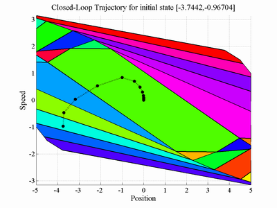
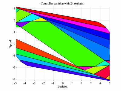
The simplot function replaces mpt_plotTrajectory and mpt_plotTimeTrajectory and can thus be used to visualize closed-loop trajectories. If the initial state x0 is not specified and the controller is in 2D, the function will allow you to specify the initial state by mouse, e.g.

>> Double_Integrator
>> ctrl = mpt_control(sysStruct, probStruct);
>> simplot(ctrl)

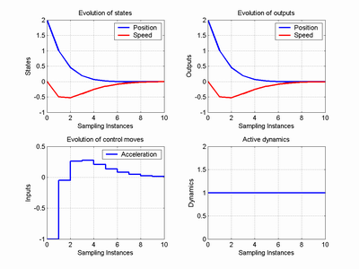
If x0 is specified, simplot will plot the evolution of states, inputs and outputs versus time, e.g.

>> Double_Integrator
>> ctrl = mpt_control(sysStruct, probStruct);
>> x0 = [2; 0];
>> simplot(ctrl, x0)

Again, it is possible to specify a different system dynamics by either providing your own sysStruct or giving a handle of a function which should be used to compute the state update:

>> Double_Integrator
>> ctrl = mpt_control(sysStruct, probStruct);
>> x0 = [2; 0];
>> simplot(ctrl, @di_sim_fun, x0)

For more information about this function, see help mptctrl/simplot.

Support for lower-dimensional noise polytopes

MPT now supports lower-dimensional noise polytopes! If you want to define noise only on a subset of system states, you can now do so by defining sysStruct.noise as a set of vertices representing the noise. Say you want to impose a +/- 0.1 noise on x1, but no noise should be used for x2. You can do that by:

>> sysStruct.noise = [-0.1 0.1; 0 0];

Just keep in mind that the noise polytope must have vertices stored column-wise.

MEX files for the GLNXA64 platform

Thanks to Marco Laumanns, MPT now includes all necessary MEX files compiled for the GLNXA64 (64-bit Linux for AMP processors) platform.

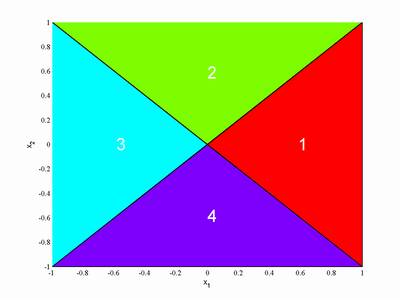
More detailed display of system structures

The command mpt_sysStructInfo is now extended to display detailed information about a given linear or hybrid systems. To use the new feature, call the function with no output arguments, e.g.

>> pwa_DI
>> mpt_sysStructInfo(sysStruct)

which will generate the following output:

  PWA system (4 dynamics), 2 states, 1 input, 2 outputs

  Guards of dynamics 1:
  x(1) >= 0
  x(2) >= 0

  Guards of dynamics 2:
  x(1) <= 0
  x(2) <= 0

  Guards of dynamics 3:
  x(1) <= 0
  x(2) >= 0

  Guards of dynamics 4:
  x(1) >= 0
  x(2) <= 0

Execute arbitrary functions on each element of a polytope array

PELEMFUN(@FHANDLE, Pn, [X1, ..., Xn]) evaluates a function defined by the function handle FHANDLE on all elements of the polytope array Pn. Additional input arguments X1,...,Xn can be specified as well. A couple of examples:

E = pelemfun(@extreme, Pn) returns the extreme points of all polytopes stored in the polytope array Pn as a cell array:

>> p = unitbox(2);
>> P = [p p+[1; 0] p+[-1; 0]];
>> E = pelemfun(@extreme, P)

E = 

    [4x2 double]    [4x2 double]    [4x2 double]
    
>> E{1}

ans =

     1    -1
     1     1
    -1     1
    -1    -1

[X, R] = pelemfun(@chebyball, Pn) returns centers and radii of the chebychev ball of each element of Pn:

>> [X, R] = pelemfun(@chebyball, P)

X = 

    [2x1 double]    [2x1 double]    [2x1 double]


R = 

    [1]    [1]    [1]

B = pelemfun(@bounding_box, Pn, struct('Voutput', 1)); V = [B{:}] returns bounding boxes of all elements of Pn converted to a matrix.

I = pelemfun(@le, Pn, Q) returns a cell array of logical statements with true value at position "i" if Pn(i) is a subset of Q:

>> I = pelemfun(@le, P, unitbox(2, 1.5)); 
>> [I{:}]

ans =

     1     0     0

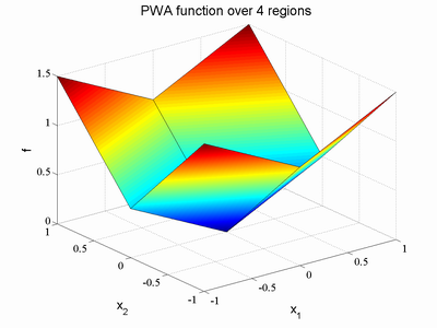
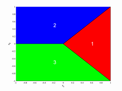
Convert a linear norm into a PWA function

The new function mpt_norm2pwa transforms a linear norm ||P*x||_l into an equivalent PWA function, ||P*x||_l = pwafcn.Bi{i}*x + pwafcn.Ci{i} for x \in pwafcn.Pn(i). Example:

>> P = diag([0.5 1]);  % scaling matrix
>> N = 1;              % transform the 1-norm
>> Pn = unitbox(2);    % only look for a solution inside of this box
>> pwafcn = mpt_norm2pwa(P, N, struct('Pn', Pn));
>> mpt_plotPWA(pwafcn.Pn, pwafcn.Bi, pwafcn.Ci);

Allow to deal with holes in explicit solutions

If a hole is present in an explicit solution, you can now tell mpt_getInput to take the control law of the nearest neighboring region if a state lies in the hole. To use this feature, you must set Options.recover=1, i.e.

>> Double_Integrator
>> ctrl = mpt_control(sysStruct, probStruct);  % compute the explicit controller
>> Pfinal = ctrl.Pfinal;                       % record feasible set
>> ctrl = modify(ctrl, 'remove', 2);           % remove 2nd region
>> ctrl = set(ctrl, 'Pfinal', Pfinal);         % set back the feasible set
>> plot(ctrl)

Here we see that our explicit controller contains a hole, so there is no control law defined for the initial state x0 = [-5; 1]:

>> u = mpt_getInput(ctrl, [-5; 1])
MPT_GETINPUT: NO REGION FOUND FOR STATE x = [-5  1]

u =

     []

However, with the recovery mode turned on, we take the control law of the nearest neighbor:

>> Options.recover = 1;
>> u = mpt_getInput(ctrl, [-5; 1], Options)
MPT_GETINPUT: State x = [-5  1] lies in a hole, taking the nearest neighbor

u =

     1

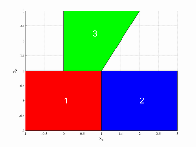
New function to compute the list of adjacent polytopes

The new function mpt_buildAdjacency now allows to compute which polytopes of a given polytope array are adjacent, i.e. which of them share a common facet. See help mpt_buildAdjacency for more details. Small example:

>> p1 = unitbox(2); 
>> p2 = unitbox(2) + [2; 0]; 
>> p3 = polytope([0 1; 0 3; 1 1; 2 3]);
>> P = [p1 p2 p3];
>> plot(P); identifyRegion(P)

>> adj = mpt_buildAdjacency(P);
>> adj{1}
ans =

     2     0
     3  -Inf
  -Inf     0
  -Inf     0

this output means that polytope p1 and polytope p2 share a common facet, so do polytopes p1 and p3.

>> adj{3}
ans =

     1
  -Inf
  -Inf
  -Inf

and this shows that polytope p3 is only adjacent to polytope p1, but not to p2. Have a look at help mpt_buildAdjacency for more information.

Improved computation of maximum attractive sets

The function mpt_maxCtrlSet has undergone a major revision:

Sets obtained at each iteration can now be returned
Computation of maximal attractive sets can now be aborted prematurely if convergence is very slow (have a look at help mpt_maxCtrlSet and look at Options.Vconverge
Custom problem structure can now be passed (Options.probStruct)

Allow to disable the construction of a simulator when importing HYSDEL models

mpt_sys now allows to disable the construction of a simulator when hybrid systems modeled by HYSDEL are imported. To use this feature, call mpt_sys with an additional 'nosimulator' input argument:

>> sysStruct = mpt_sys('hysdelfile', 'nosimulator')

This is especially handy when you want to use the generated model only for on-line MPC of systems which are not well defined.

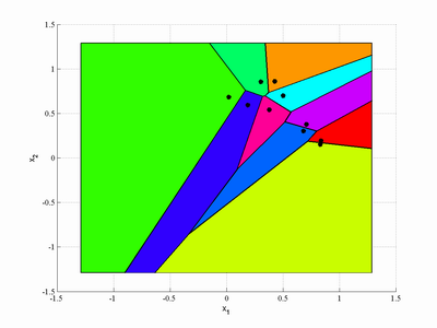
Sort voronoi cells according to seed points

P=mpt_voronoi(S) now returns the regions sorted in a way such that region P(i) corresponds to seed point S(i, :). Example:

>> S = rand(5, 2);      % 5 random seed points in 2D
>> V = mpt_voronoi(S);  % compute the voronoi cells
>> [isin, inwhich] = isinside(V, S(1, :)'); inwhich

inwhich =

1

>> [isin, inwhich] = isinside(V, S(2, :)'); inwhich

inwhich =

2

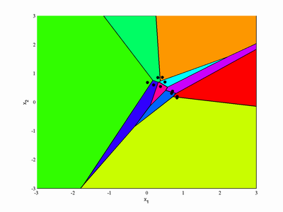
Allow to specify a "bounding polytope" when computing Voronoi cells

P=mpt_voronoi(S) now allows you to specify a "bounding polytope", i.e. the polytope inside of which the Voronoi cells should be computed.

% generate 10 random seed points in 2D
>> S = rand(10, 2);  

% compute voronoi cells without specifying a bounding polytope
>> V = mpt_voronoi(S);

% look for solution inside of a box with sides of +/- 3
>> Options.pbound = unitbox(2, 3);

% compute the Voronoi cells
>> P = mpt_voronoi(S);

Allow to specify the type of Lyapunov function to compute for one-step controllers

When constructing a one-step solution for PWA systems (probStruct.subopt_lev=2), MPT now allows to specify which type of Lyapunov function should be used to testify stability of the closed-loop system. The Lyapunov function can now be specified in Options.lyapunov_type which can take the following strings:

Options.lyapunov_type='any' - let MPT decide which one to use (usually a PWQ Lyapunov function will be used
Options.lyapunov_type='pwq' - compute a Piecewise Quadratic Lyapunov function
Options.lyapunov_type='pwa' - compute a Piecewise Affine Lyapunov function
Options.lyapunov_type='none' - don't compute any Lyapunov function (the closed-loop system can be unstable!)

Easy detection of overlaps

Assume you have a polytope array and want to find out which polytopes do intersect. Now you can do

>> p1 = unitbox(2);
>> p2 = unitbox(2)+[1; 0];
>> p3 = unitbox(2)+[-1; 0];
>> p = [p1 p2 p3];
>> [r, ia, ib, iab] = dointersect(P, P);
>> iab

iab =

     1     1
     1     2
     1     3
     2     1
     2     2
     3     1
     3     3

and this output tells you that p1 intersects with p2 and p3, but p2 does not intersect with p3.

Improved `facetcircle` function

polytope/facetcircle now allows to pass the whole range of facets to explore, e.g:

>> P = unitbox(3);
>> [x, r] = facetcircle(P, [1 3])

x =

     1     0
     0     0
     0     1


r =

     1     1

Notice that the centers of facets nos. 1 and 3 returned in x are stored column-wise.

Function to compute a voronoi diagram for facets of a polytope

Similar to the idea of Voronoi diagrams one can compute the partition of a polytope for which the set of points in a polytope is closer to one facet than to all the others:

>> P = unitbox(2);
>> V = facetvoronoi(P)
V=

Polytope array: 4 polytopes in 2D

>> plot(V)

Here V(i) is a polytope which contains all points which are closer to facet no. i of P than to any other facet. A subset of facets to investigate can also be provided:

>> P = unitbox(2);
>> V = facetvoronoi(P, [1 2 4])
V=

Polytope array: 3 polytopes in 2D

>> plot(V)

New function to remove redundant entries of a polytope array

If your polytope array contains duplicate elements, you can now use the overloaded function unique which will return only unique elements of the array:

>> p1 = unitbox(2);
>> p2 = unitbox(2, 5);
>> P = [p1 p2 p1 p1 p2]    % P contains redundant entries

P=

Polytope array: 5 polytopes in 2D

>> U = unique(P)

U=

Polytope array: 2 polytopes in 2D

>> U(1)==p1

ans =

     1
     
>> U(2)==p2
 
ans =

     1

Improved projection algorithms

A new projection method has been added - Options.projection=7. When this algorithm is selected, the projection is solved as a multi-parametric linear program (mpLP). This method is efficient especially when projecting to, say, less than 5 dimensions. We have also improved other algorithms, mainly increased numerical robustness of the ESP method (Options.projection=4) and changed heuristics which decides which projection method best suits a particular problem.

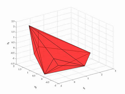
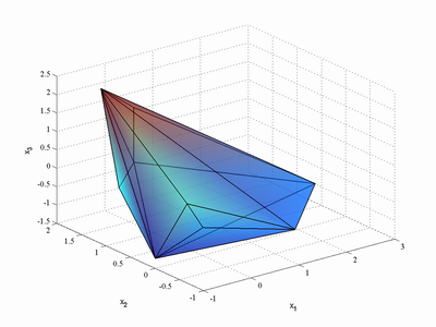
New options for plotting of polytopes

Gradient coloring can now be used when plotting 3D polytopes:

>> P = polytope(randn(10,3));
>> plot(P); % plot with gradient coloring disabled

>> plot(P, struct('gradcolor', 1)); % plot with gradient coloring enabled

Moreover, a colormap can now be specified when plotting polytope arrays:

>> plot(Pn, struct('colormap', 'summer'));

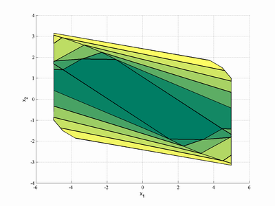
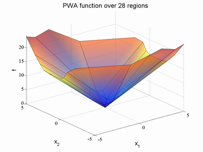
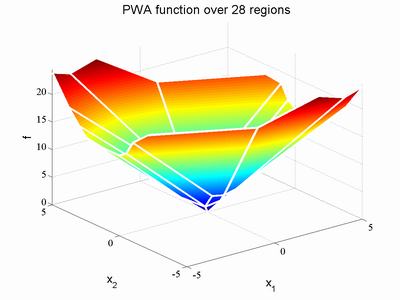
Improved plotting of piecewise affine and piecewise quadratic functions

Functions mpt_plotPWA and mpt_plotPWQ have been extended to allow the user to specify color of edges of patches (Options.edgecolor) and level of transparency (Options.shade). The width of edge lines can be specified by Options.edgewidth. Have a look at respective help descriptions for more details.

>> mpt_plotPWA(Pn, Li, Ci, struct('shade', 0.6));

>> mpt_plotPWQ(Pn, Li, Ci, struct('edgecolor', 'w', 'edgewidth', 3));

Notable changes and bug fixes in the polytope library

polytope/bounding_box: allows to return all vertices of a bounding box
polytope/bounding_box: change behavior with Options.noPolyOutput


    polytope/extreme: allow rounding to increase numerical
    robustness for CDD (Options.roundat)
    polytope/facetcircle: properly normalize vectors of normals
    polytope/minus, polytope/plus: treat polytope arrays as a union
    of polytopes, not as single polytopes
    polytope/mtimes: allow scaling even when origin is not included 
    polytope/plot: supports Options.zvalue 
    polytope/projection: fix problems with fourier-motzkin
    C-implementation
    polytope/projection: fix handling of dimensions which are not sorted 
    polytope/reduce: always return correct keptrows 
    polytope/reduce: preserve order of hyperplanes
    polytope/regiondiff: fix problems with Options.infbox being too
    large
    polytope/triangulate: properly update extreme points
    polytope/triangulate, polytope/volume: do not return 
    volume as a complex number



Other notable changes and bug fixes


    mpt_computeTrajectory fixed computation of closed-loop cost for
    systems with deltaU constraints
    mpt_exportc: allows to specify name of output file 
    
    mpt_getInput: don't check regions twice
    
    
    mpt_infsetPWA: properly detect cases where invariant set is empty 
    
    
    mpt_invariantSet: speed improvements 
    
    
    mpt_invariantSet: allow to simplify intermediate steps using
    greedy merging 
    
    
    mpt_init: improve speed
    
    
    mpt_mplp: fix problems with cycling 
    
    
    mpt_mplp: fix random perturbations for 1D systems 
    
    
    mpt_mplp: fix problems with "xBeyond violates more than one bounds" 
    
    
    mpt_mpqp: improved handling of degeneracies
    
    
    mpt_optControlPWA: fixed handling of 1D systems 
    
    
    mpt_optControlPWA: always return Pfinal as a polytope array 
        
    
    mpt_plotPWA, mpt_plotPartition, 
    mpt_plotU: respect user's choice of subplots 
    
    
    mpt_plotU: fixed handling of 1D systems with multiple inputs 
    
    
    mpt_solveQP: properly impose equality constraints for NAG QP solver 
    
    
    mpt_voronoi: make mpt_mplp() silent